Absolute Value Equations 1 Directions Absolute Value

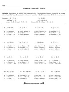
ABSOLUTE VALUE EQUATIONS #1 Directions absolute …

ABSOLUTE VALUE EQUATIONS #1. Directions: Solve each of the absolute value equations below. Test each possible solution by replacing the variable with each possible value. For your answer choose the values that make the equation true. Circle the correct answer. Examples: x + = 7 10 x − = 2 22 x = 3 and x = -17 x = 24 and x = -20

  Value, Directions, Equations, Absolute, Absolute value equations, 1 directions absolute

Lecture #7 Lagrange's Equations - MIT OpenCourseWare

Have 2 differential equations of constraint, neither of which can be integrated without solving the entire problem. Constraints are nonholonomic Reason? Can relate change in θ to change in x,y for given φ, but the absolute value of θ depends on the path taken to …

  Value, Equations, Absolute, Mit opencourseware, Opencourseware, Absolute value

The node voltage method - Iowa State University

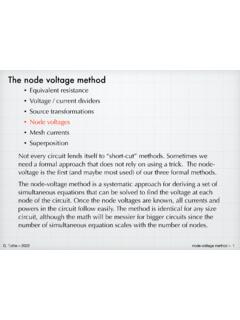
EE 201 node-voltage method – 5 Voltage, like energy, is a relative quantity — only differences are important. The absolute values of v a, v b, v c,and v d do not matter — only the differences, v a – v b, v a – v c, etc. are important, as we saw in the previous set of equations.

  Equations, Absolute, Voltage

Chapter 1 Governing Equations of Fluid Flow and Heat Transfer

equations (conservation of mass, 3 components of conservation of momentum, conservation of energy and equation of state). 1.4 Incompressible Flows For incompressible flows density has a known constant value, i.e. it is no longer an unknown. Also for an incompressible fluid it is not possible to talk about an equation of state.

  Value, Equations

Singular Value Decomposition (SVD)

Singular value Decomposition t i i r i ii A USV T ¦ S u v 1 This m by n matrix u i vT i is the product of a column vector u i and the transpose of column vector v i. It has rank 1. Thus A is a weighted summation of r rank-1 matrices. Note: u i and v i are the i …

  Value, Singular, Decomposition, Singular value decomposition

Water Pressure and Pressure Forces - Pearson

The pressure at points 1 and 2 must be the same since the system is in static equilibrium. Step 3. (a) For open manometers, the pressure on 2 is exerted by the weight of the liquid M column above 2; and the pressure on 1 is exerted by the weight of the col-umn of water above 1 plus the pressure in vessel A. The pressures must be equal in value.

  Pressure, Water, Value, Force, Water pressure and pressure forces

Chapter 11 Density of States, Fermi Energy and Energy Bands

11-3 ! p k (11.6) Knowing the momentum p = mv, the possible energy states of a free electron is obtained m k m p E mv 2 2 2 1 2 2 ! (11.7) which is called the dispersion relation (energy or frequency-wavevector relation). Effective Mass In reality, an electron in a crystal experiences complex forces from the ionized atoms.

Lecture Notes on General Relativity Columbia University

g= dt2 + (dx1)2 + (dx2)2 + (dx3)2: (1.1) Note that (for an arbitrary pseudo-Riemannian metric) one can still introduce a Levi{Civita connection and therefore de ne the notion the associated Christo el symbols and geodesic

  Lecture, Notes, General, Relativity, Lecture notes on general relativity

General Relativity

CONTENTS 5 Introduction General Relativity is the classical theory that describes the evolution of systems under the e ect of gravity. Its history goes back to …

Matthew Schwartz Lecture 3: Coupled oscillators

Behavior starting from x1=1,x0=0 Normal mode behavior Figure 1. Left shows the motion of masses m=1,κ=2 and k =4 starting with x1=1 and x2=0. Right shows the normal modes, with x1=x2=1(top) and x1=1,x2=−1(bottom). If you look closely at the left plot, you can make out two distinct frequencies: the normal mode frequencies, as shown on the right.

  Oscillators, Coupled, Coupled oscillators