
Chapter 3
22 3. Continuous Functions If c ∈ A is an accumulation point of A, then continuity of f at c is equivalent to the condition that lim x!c f(x) = f(c), meaning that the limit of f as x → c exists and is equal to the value of f at c. Example 3.3. If f: (a,b) → R is defined on an open interval, then f is continuous on (a,b) if and only iflim x!c f(x) = f(c) for every a < c < b ...
Download Chapter 3

Information
Domain:
Source:
Link to this page:
Documents from same domain

LECTURE 5 - UC Davis Mathematics
www.math.ucdavis.eduLECTURE 5. STOCHASTIC PROCESSES 133 We say that random variables X 1;X 2;:::X n: !R are jointly continuous if there is a joint probability density function p(x
A concise introduction to quantum probability, …
www.math.ucdavis.eduA concise introduction to quantum probability, quantum mechanics, and ... precepts of quantum mechanics are sometimes called ... This article is a concise introduction to quantum probability theory, quantum mechanics, and quan-tum computation for the mathematically prepared
An introduction to quantum probability, quantum …
www.math.ucdavis.eduAn introduction to quantum probability, quantum mechanics, and quantum computation Greg Kuperberg∗ UC Davis (Dated: October 8, 2007) Quantum mechanics is one of the most surprising

Linear Algebra in Twenty Five Lectures
www.math.ucdavis.eduThese linear algebra lecture notes are designed to be presented as twenty ve, fty minute lectures suitable for sophomores likely to use the material for applications but still requiring a solid foundation in this fundamental branch
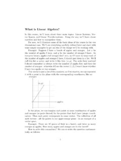
What is Linear Algebra? - University of California, …
www.math.ucdavis.eduWhat is Linear Algebra? In this course, we’ll learn about three main topics: Linear Systems, Vec-tor Spaces, and Linear Transformations. Along the way we’ll learn about
Twenty problems in probability - UC Davis …
www.math.ucdavis.eduTwenty problems in probability This section is a selection of famous probability puzzles, job interview questions (most high- tech companies ask their applicants math questions) and math competition problems.
Complex Analysis Lecture Notes - UC Davis Mathematics
www.math.ucdavis.edu\entropy"), and lots of applications to things that seem unrelated to complex numbers, for example: Solving cubic equations that have only real roots (historically, this was the
David Cherney, Tom Denton, Rohit Thomas and Andrew …
www.math.ucdavis.eduLinear algebra is the study of vectors and linear functions. In broad terms, vectors are things you can add and linear functions are functions of vectors that respect vector addition.
Power Series - UC Davis Mathematics :: Home
www.math.ucdavis.eduThe power series in Definition 6.1 is a formal expression, since we have not said anything about its convergence. By changing variables x→ ( x−c ), we can assume
LECTURE NOTES ON APPLIED MATHEMATICS
www.math.ucdavis.eduLECTURE 1 Introduction The source of all great mathematics is the special case, the con-crete example. It is frequent in mathematics that every instance
Related documents

Graphing Polynomial Functions
static.bigideasmath.comSection 4.1 Graphing Polynomial Functions 161 Solving a Real-Life Problem The estimated number V (in thousands) of electric vehicles in use in the United States can be modeled by the polynomial function V(t) = 0.151280t3 − 3.28234t2 + 23.7565t − 2.041 where t represents the year, with t = 1 corresponding to 2001. a. Use a graphing calculator to graph the function for …
Unit 3 Chapter 6 Polynomials and Polynomial Functions
www.scasd.orgCP A2 Unit 3 Ch 6 Worksheets and Warm Ups 1 Unit 3 – Chapter 6 Polynomials and Polynomial Functions Worksheet Packet Mrs. Linda Gattis LHG11@scasd.org Learning Targets: Polynomials: The Basics 1. I can classify polynomials by degree and number of terms. 2. I can use polynomial functions to model real life situations and make predictions 3.
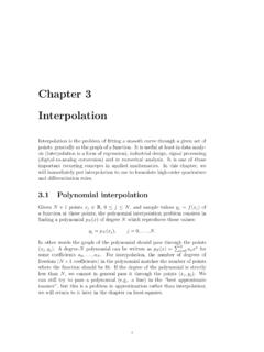
Chapter 3 Interpolation - MIT OpenCourseWare
ocw.mit.eduIn this chapter, we will immediately put interpolation to use to formulate high-order quadrature and di erentiation rules. 3.1 Polynomial interpolation Given N+ 1 points x j 2R, 0 j N, and sample values y j = f(x j) of a function at these points, the polynomial interpolation problem consists in nding a polynomial p
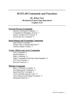
MATLAB Commands and Functions - Omicron Chapter
www.hkn.umn.eduPolynomial and Regression Functions / 14 Interpolation Functions / 14 Numerical Integration Functions / 14 Numerical Differentiation Functions / 14 ODE Solvers / 15 Predefined Input Functions / 15 Symbolic Math Toolbox Functions for Creating and Evaluating Symbolic Expressions / 16

Chapter 3 Polynomial Functions - MS Guides
wp.srsd119.caChapter 3 Polynomial Functions Section 3.1 Characteristics of Polynomial Functions Section 3.1 Page 114 Question 1 A polynomial function has the form f(x) = anx n + a n – 1x n – 1 + a n – 2x n – 2 + … + a 2x 2 + a 1x + a0, where an is the leading coefficient; a0 is the constant; and the degree of the polynomial, n,
Chapter 3 Interpolation - MathWorks
www.mathworks.com2 Chapter 3. Interpolation There are n terms in the sum and n − 1 terms in each product, so this expression defines a polynomial of degree at most n−1.If P(x) is evaluated at x = xk, all the products except the kth are zero.Furthermore, the kth product is equal to one, so the sum is equal to yk and the interpolation conditions are satisfied. For example, consider the following data set.

Chapter 5 Techniques of Differentiation
www.math.smith.eduWe also saw in chapter 3 that the polynomial 5x3−7x2+3 can be thought of as an algebraic combination of simple functions. We can build an even...and algebraically more complicated function by forming a quotient with this polynomial in the numerator and the difference of the functions sinx and ex in the denominator. The result is 5x3 − 7x2 ...

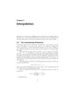
Chapter 3 - Interpolation
www.cs.usask.ca3.1 The Interpolating Polynomial Interpolationis the process of de ning a function that \connects the dots" between speci ed (data) points. In this chapter, we focus on two closely related interpolants, thecubic splineand theshape-preserving cubic splinecalled \pchip". Two distinct points uniquely determine a straight line.

Unit 3 (Ch 6) Polynomials and Polynomial Functions
www.scasd.orgCP A2 Unit 3 (chapter 6) Notes 11 LT2. I can use polynomial functions to model real life situations and make predictions Comparing Models Use a graphing calculator to find the best regression equation for the following data. Compare linear, quadratic and cubic regressions.