
CHAPTER 3: Random Variables and Probability Distributions
1=2 if 4 x < 6 5=6 if 6 x < 10 1 if x 10; nd the probability mass function. Solution: Continuous Probability Distribution: 3.3 A density curve is a curve that is always on or above the horizontal axis, and has area exactly 1 underneath it. A density curve describes the overall pattern of a distribution. The area under the curve and above any
Download CHAPTER 3: Random Variables and Probability Distributions

Information
Domain:
Source:
Link to this page:
Documents from same domain
STAT 1030 Business Statistics Additional Final Exam ...
homepage.divms.uiowa.eduSTAT 1030 Business Statistics Additional Final Exam Practice Questions (Part II) Contributed by former TA Scott Wood (also nicknamed "Scooter") 1
Biostatistics 22S:101 Answers to Practice Exam 2
homepage.divms.uiowa.eduBiostatistics 22S:101 Answers to Practice Exam 2 1. A large population contains an unknown proportion (p) of black marbles. A sample of n=200 drawn scientifically

XSL Transformations - University of Iowa
homepage.divms.uiowa.eduXSLT supplies another way to perform these kinds of tasks. XSL (Extensible Stylesheet Language) is an application of XML that provides tools for transforming an XML document
NUMERICALSOLUTIONOF ORDINARYDIFFERENTIAL …
homepage.divms.uiowa.eduNUMERICALSOLUTIONOF ORDINARYDIFFERENTIAL EQUATIONS Kendall Atkinson, Weimin Han, David Stewart ... 3.1 Higher-order differential equations 39 3.2 Numerical methods for systems 42 ... methods for solving boundary value problems of second-order ordinary differential equations. The final chapter, Chapter12, gives an introduct ionto the numerical ...

FIXED POINT ITERATION
homepage.divms.uiowa.eduIn general, we are interested in solving the equation x = g(x) by means of xed point iteration: x ... The statement x n+1 ˇg0( )( x n) ... This is an approximation to Newton’s method, with f0(x n) ˇD n. To analyze its convergence, regard it as a xed point iteration with
NUMERICALSOLUTIONOF ORDINARYDIFFERENTIAL …
homepage.divms.uiowa.edu8.5 Solving the finite-difference method 145 8.6 Computer codes 146 Problems 147 9 Implicit RK methods for stiff differential equations 149 9.1 Families of implicit Runge–Kutta methods 149 9.2 Stability of Runge–Kutta methods 154 9.3 Order reduction 156 9.4 Runge–Kutta methods for stiff equations in practice 160 Problems 161

3.6 Exercises
homepage.divms.uiowa.edu3.6 Exercises 47 (d) Suppose computers are repeatedly selected (assume independence). Find the probability that the 4th selected computer is the first one running Linux. 3.14 A slot machine has 3 wheels. Each wheel has 10 symbols, and each symbol is equally likely when the wheel is spun (assume the wheels act independently of each other). The
LEAST SQUARES APPROXIMATION - University of Iowa
homepage.divms.uiowa.edugis a quadratic polynomial in the two variables ... ulating this set of conditions leads to a simultaneous linear system. To better understand the form of the linear system, consider the special case of [a,b]=[0,1]. Differenti-ating gwith respect to each ...

A Brief History of Statistics (Selected Topics)
homepage.divms.uiowa.eduthe ancient Greeks – Extended to more than two numbers in the late 1500s in ... milestones in the history of science, and it became a staple in astronomy and other physical sciences by the mid-1800s. • It took until about 1900 before it had fully diffused into other scientific disciplines 11. Some important figures after Laplace and Gauss
Related documents
Chapter 5: JOINT PROBABILITY DISTRIBUTIONS Part 1 ...
homepage.stat.uiowa.eduThere are 6 possible pairs (X;Y). We show the probability for each pair in the following table: x=length 129 130 131 y=width 15 0.12 0.42 0.06 16 0.08 0.28 0.04
Chapter 7 Continuous Distributions - Yale University
www.stat.yale.edu7. Continuous Distributions 5 Example <7.5> Zero probability for ties with continuous distributions. Calculations are also greatly simpli ed by the fact that we can ignore contributions from higher order terms when working with continuous distri-butions and small intervals. Example <7.6> The distribution of the order statistics from the uniform
Chapter 5: Discrete Probability Distributions
coconino.eduChapter 5: Discrete Probability Distributions 158 This is a probability distribution since you have the x value and the probabilities that go with it, all of the probabilities are between zero and one, and the sum of all of the probabilities is one. You can give a probability distribution in table form (as in table #5.1.1) or as a graph.
Chapter 6: Continuous Probability Distributions
coconino.eduChapter 6: Continuous Probability Distributions 193 Section 6.3: Finding Probabilities for the Normal Distribution The Empirical Rule is just an approximation and only works for certain values. What if you want to find the probability for x values that are not integer multiples of the standard deviation? The probability is the area under the curve.
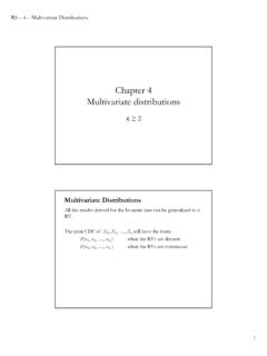
Chapter 4 Multivariate distributions
www.bauer.uh.eduRS – 4 – Multivariate Distributions 1 Chapter 4 Multivariate distributions k ≥2 Multivariate Distributions All the results derived for the bivariate case can be generalized to n RV. The joint CDF of X1, X2, …, Xk will have the form: P(x1, x2, …, xk) when the RVs are discrete F(x1, x2, …, xk) when the RVs are continuous

Chapter 3 Continuous Random Variables
www.pnw.eduChapter 3 Continuous Random Variables ... Figure 3.1: Comparing discrete and continuous distributions 73. 74 Chapter 3. Continuous Random Variables (LECTURE NOTES 5) ... Random variable Xis continuous if probability density function (pdf) fis continuous at all but a nite number of points and possesses the following properties: f(x) 0, for all x,
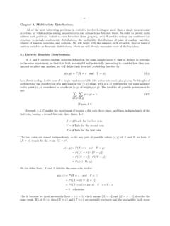
Chapter 3. Multivariate Distributions.
www.stat.uchicago.eduChapter 3. Multivariate Distributions. ... structure to include multivariate distributions, the probability distributions of pairs of random variables, triplets of random variables, and so forth. ... satisfying (3.10) and (3.11) describes a continuous bivariate probability distribution. It can help the intuition to think of a continuous ...