Finite Difference Method for Solving Differential Equations

Chapter 01.03 Sources of Error - MATH FOR COLLEGE

01.03.1 Chapter 01.03 Sources of Error After reading this chapter, you should be able to: 1. know that there are two inherent sources of error in numerical methods – round-

  Methods, Chapter, Course, Numerical, Chapter 10, Errors, Numerical methods, 03 sources of error

Runge-Kutta 4th Order Method for Ordinary …

08.04.1 Chapter 08.04 Runge-Kutta 4th Order Method for Ordinary Differential Equations . After reading this chapter, you should be able to . 1. develop Runge-Kutta 4th order method for solving ordinary differential equations,

  Methods, Order, Differential, Equations, Ordinary, Order method for ordinary, Order method for ordinary differential equations

Simpson 3/8 Rule for Integration - MATH FOR …

In a similar fashion, Simpson rule for integration can be derived by 3/8 approximating the given function

  Rules, Integration, Simpsons, Simpson 3 8 rule for integration

Finite Difference Method for Solving Differential …

08.07.1 . Chapter 08.07 Finite Difference Method for Ordinary Differential Equations . After reading this chapter, you should be able to . 1. Understand what the finite difference method is and how to use it to solve problems.

  Methods, Solving, Differences, Finite, Finite difference method, Finite difference method for solving

Chapter 04.08 Gauss-Seidel Method

using the Gauss-Seidel method. Assume an initial guess of the solution as = 5 2 1

  Methods

Chapter 05.03 Newton’s Divided Difference Interpolation

Newton’s Divided Difference Interpolation 05.03.3 Figure 2 Linear interpolation. Example 1 The upward velocity of a rocket is given as a function of time in Table 1 (Figure 3).

  Differences, Divided, Newton, Interpolation, Newton s divided difference interpolation

False-Position Method of Solving a Nonlinear Equation

03.06.1 . Chapter 03.06 False-Position Method of Solving a Nonlinear Equation . After reading this chapter, you should be able to . 1. follow the algorithm of the false-position method of solving a nonlinear equation,

  Methods, Position, Solving, False, False position method

Bisection Method of Solving Nonlinear Equations: General ...

One of the first numerical methods developed to find the root of a nonlinear equation . f (x) =0 was the bisection method (also called binary-search method). The method is based on the following theorem. Theorem. An equation. f (x) =0, where f (x) is a real continuous function, has at least one root between . x and . x. u. if f (x ) f (x. u ...

  Methods, Numerical, Numerical methods, Bisection method, Bisection

Runge-Kutta 4th Order Method for Ordinary Differential ...

Oct 13, 2010 · 08.04.1 Chapter 08.04 Runge-Kutta 4th Order Method for Ordinary Differential Equations . After reading this chapter, you should be able to . 1. develop Runge-Kutta 4th order method for solving ordinary differential equations, 2. find the effect size of step size has on the solution, 3. know the formulas for other versions of the Runge-Kutta 4th order method

  Order, Differential, Runge, Kutta, Runge kutta

Chapter 10.02 Parabolic Partial Differential Equations

Parabolic Partial Differential Equations . After reading this chapter, you should be able to: 1. Use numerical methods to solve parabolic partial differential eqplicit, uations by ex implicit, and Crank-Nicolson methods. The general second order linear PDE with two independent variables and one dependent variable is given by . 0. 2 2 2 2 2 ...

  Differential, Equations, Differential equations, Parabolics

FINITE ELEMENT METHOD

1. Finite Difference Method (FDM) 2. Finite Volume Method (FVM) 3. Finite Element Method (FEM) 4. Boundary Element Method (BEM) 5. Spectral Method 6. Perturbation Method (especially useful if the equation contains a small parameter) 1.1 Finite Difference Method The finite difference method is the easiest method to understand and apply.

  Methods, Differences, Difference method

The Effect of Inquiry -based Learning Method on Students ...

relationship between the method of instruction and the attainment of objectives (Baez, 1971). Among these different kinds of methodologies, inquiry method has an important place. The inquirybased teaching approach is supported on - knowledge about the learning process t hat has emerged from research (Bransford, Brown, & Cocking, 2000). In

  Methods

Finite Difference Methods - Massachusetts Institute of ...

Example 1. Finite Difference Method applied to 1-D Convection In this example, we solve the 1-D convection equation, ∂U ∂t +u ∂U ∂x =0, using a central difference spatial approximation with a forward Euler time integration, Un+1 i −U n i ∆t +un i δ2xU n i =0.

  Methods, Differences, Difference method

Understanding the Finite-Difference Time-Domain Method

on the finite-difference time-domain (FDTD) method. The FDTD method makes approximations that force the solutions to be approximate, i.e., the method is inherently approximate. The results obtained from the FDTD method would be approximate even if we used computers that offered infinite numeric precision.

  Methods, Differences, Finite, Finite difference, Fdtd, Fdtd method

Solving Linear Programs 2

simplex method, proceeds by moving from one feasible solution to another, at each step improving the value of the objective function. Moreover, the method terminates after a finite number of such transitions. Two characteristics of the simplex method have led to its widespread acceptance as a computational tool. First, the method is robust.

  Methods

Introductory Finite Difference Methods for PDEs

Introductory Finite Difference Methods for PDEs Contents Contents Preface 9 1. Introduction 10 1.1 Partial Differential Equations 10 1.2 Solution to a Partial Differential Equation 10 1.3 PDE Models 11 &ODVVL¿FDWLRQRI3'(V 'LVFUHWH1RWDWLRQ &KHFNLQJ5HVXOWV ([HUFLVH 2. Fundamentals 17 2.1 Taylor s Theorem 17

  Methods, Differences, Introductory, Finite, Introductory finite difference methods for

Finite Di erence Methods for Di erential Equations

Finite Di erence Methods for Di erential Equations Randall J. LeVeque DRAFT VERSION for use in the course AMath 585{586 University of Washington Version of September, 2005

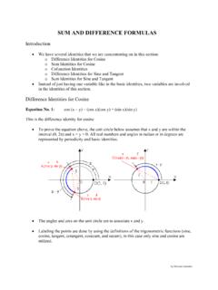
SUM AND DIFFERENCE FORMULAS - Alamo Colleges District

• From the difference identity for cosine equation, we are going to attain the cofunction ... cos x and sin y, let’s do the Unit Circle method. • sin x = -1/3 and x is in quadrant III, let’s find cos x: by Shavana Gonzalez . Example 3 (Continued): cos x = a . a2 + b2 = 1 .

  Methods, District, College, Differences, Omala, Alamo colleges district

Method of Standard Additions (MSA/SA)

difference from the original standard curve. 2. Effect of the interference should not vary as the ratio of analyte conc. to sample matrix changes, and the SA should respond in a similar manner as the analyte. 3. Must be free of spectral interference and corrected for nonspecific background interference. Ref:SW-846 7000B, Section 8.7 & 7010 ...

  Methods, Differences