Integration and Differential Equations

A Brief Review of Elementary Ordinary Differential …

Review of Elementary ODEs 6 Second-Order Linear Homogeneous Equations with Constant Coefficients§ Consider a differential equation of the form ay′′ + by′ + cy = 0 where a, b, and c are (real) constants.

  Review, Differential, Equations, Ordinary, Elementary, Review of elementary ordinary differential

Answers to Selected Exercises - University of Alabama in ...

Answers to Selected Exercises Chapter 1 1. second, fifth, fifth, forty-second 3a i. yes, it is 3a ii. no, it is not 3a iii. no 3b i. no 3b ii. yes 3b iii. no 3c i. yes 3c ii. no 3c iii. no 3d i. no

  Exercise, Answers, Selected, Answers to selected exercises

Reduction of Order - University of Alabama in Huntsville

Reduction of Order for Homogeneous Linear Second-Order Equations 285 Thus, one solution to the above differential equation is y 1(x) = x2. As alreadystated,this method is forfinding a generalsolutionto some homogeneous linear

  Reduction, Second, Order, Differential, Equations, Order equations, Reduction of order

Sturm-Liouville Problems

Sturm-Liouville Problems “Sturm-Liouvilleproblems”areboundary-valueproblemsthat naturallyarisewhen solvingcer-tain partial differential equation problems using a “separation of variables” method that will be discussed in a later chapter. It is the theory behind Sturm-Liouville problems that, …

  Problem, Sturm, Liouville, Sturm liouville problems, Sturm liouvilleproblems, Liouvilleproblems

The Inverse Laplace Transform

The fact that the inverse Laplace transform is linear follows immediately from the linearity of the Laplace transform. To see that, let us consider L−1[αF(s)+βG(s)] where α and β are any two constants and F and G are any two functions for which inverse Laplace transforms

  Transform, Inverse, Laplace, The laplace transform, The inverse laplace transform

Nonlinear Autonomous Systems of Differential Equations

Apr 11, 2014 · Chapter & Page: 43–4 Nonlinear Autonomous Systems of Differential Equations You may have encountered this creature (or its determinant) in other courses involving “two functions of two variables” or “multidimensional change of variables”. It will, in a few pages, provide a link between nonlinear and linear systems.

  System, Equations, Variable, Nonlinear, Two variables

Differentiation and the Laplace Transform

We will confirm that this is valid reasoning when we discuss the “inverse Laplace transform” in the next chapter. In general, it is fairly easy to find the Laplace transform of the solution to an initial-value problem involving a linear differential equation with constant coefficients and a ‘reasonable’ forcing function1. Simply take ...

  Transform, Inverse, Laplace transforms, Laplace, The inverse laplace transform

Partial Differential Equations I: Basics and Separable ...

Mar 08, 2014 · Ordinary Differential Equations, Appendex A of these notes. We will be using some of the material discussed there.) 18.1 Intro and Examples Simple Examples If we have a horizontally stretched string vibrating up and down, let u(x,t) = the vertical position at time t of the bit of string at horizontal position x ,

  Differential, Equations, Differential equations

Convolution - University of Alabama in Huntsville

Letusstartwithjustseeingwhat“convolution”is. Afterthat,we’lldiscussusingitwiththe Laplace transform and in solving differential equations. 27.1 Convolution, the Basics Definition and Notation Let f (t) and g(t) be two functions. The convolution of f and g , denoted by f ∗ g , is the function on t ≥ 0 given by f ∗ g(t) = Z t x=0 f ...

  Convolutions, Transform, Laplace transforms, Laplace

Sturm-Liouville Problems

It is the theory behind Sturm-Liouville problems that, ultimately, justifies the “separation of variables” method for these partial differential equation problems. The simplest applications lead to the various Fourier series, and less simple applications lead to generalizations

  Liouville

4.8 Instrumental Variables

dy=dz dx=dz: (4.46) This approach to identication of the causal parameter is given in Heckman (2000, p.58); see also the example in chapter 2.4.2. All that remains is consistent estimation of dy=dz and dx=dz. The obvi-ous way to estimate dy=dz is by OLS regression of y on z with slope estimate (z0z) 1z0y. Similarly estimate dx=dz by OLS ...

Review of First- and Second-Order System Response 1 First ...

dy dt +y(t) = f(t) (1) where the system is deflned by the single parameter ¿, the system time constant, and f(t) is a forcing function. For example, if the system is described by a linear flrst-order state equation and an associated output equation: x_ = ax+bu (2) y = cx+du: (3) and the selected output variable is the state-variable, that is ...

Differential Equations I

dy dx 3 + d4y dx4 +y = 2sin(x)+cos3(x), ... mathematical model. Using techniques we will study in this course (see §3.2, Chapter 3), we will discover that the general solution of this equation is given by the equation x = Aekt, for some constant A. We are told that x = 50 when

  Model

Lecture 4: Exponential family of distributions and ...

Generalized linear model (GLM) Various GLM models 1 Exponential family of distributions In this section, we study a family of probability distribution called the exponential family (of distributions). It is of a special form, but most, if not ... e yI(y 0)dy; it is already in the canonical form given as in (1). (3)Normal distribution ...

  Model

Gaussian Plumes from “Point” Sources

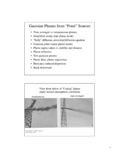
Simple Model #2: x z y X is the time-averaged wind direction, Y is the cross-wind direction, Z is the vertical dimension ( )( ) = [−] 3 m/sec m2 µg/sec m µg Gaussian Plume Model 1 2 In order to derive an equation describing the distribution of mass within the plume, we must first consider the transport of mass within a small control volume

  Form, Model, Course, Points, Gaussian, Plume, Gaussian plumes from point sources

1.3 Technology Acceptance Model 1.4 The Elements of ...

Research model based on Technology Acceptance Model (TAM) was designed by Davis (1989). The aim of the TAM was to explain theoretically the determinants factors of acceptance of computer and be efficient to make explanation for wide range of users’ behaviors. The researchers can prefer this model both estimate users’ behaviors and make

  Model

User’s Model DY Vortex Flowmeter Model DYA Vortex Flow ...

User’s Manual Model DY Vortex Flowmeter Model DYA Vortex Flow Converter FOUNDATION Fieldbus Communication Type IM 01F06F00-01EN IM 01F06F00-01EN 7th Edition

  Model, Model dy

Predator-Prey Models

• Model expressed as coupled differential equations:" AxBxy dt dx =− CyDxy dt dy =−+ The Lotka-Volterra Model cont." • Example: Rabbits and Lynxes (bobcats):" – Rabbits reproduce at a rate proportional to their population. Let x denote the number (density) of rabbits."

  Model

Topic 1: The Solow Model of Economic Growth

The rst model that we will look at in this class, a model of economic growth originally developed by MIT’s Robert Solow in the 1950s, is a good example of this general approach. Solow’s purpose in developing the model was to deliberately ignore some important aspects ofmacroeconomics, suchasshort-run

  Model