Lecture 18 Solving Shortest Path Problem: Dijkstra’s Algorithm

Lecture 16 Network Models: Minimal Spanning Tree

Lecture 16 Outline • Network Models • Minimal Spanning Tree Problem - TODAY • Shortest Route Problem • Maximal-flow Problem Operations Research Methods 1

  Lecture, Research, Network, Operations, Model, Tree, Spanning, Minimal, Operations research, Network models, Minimal spanning tree, Network models minimal spanning tree

Random Processes for Engineers 1 - University Of Illinois

1.2 Independence and conditional probability 5 1.3 Random variables and their distribution 8 ... 8.4 Baseband random processes 275 8.5 Narrowband random processes 278 8.6 Complexi cation, Part II 285 ... Stationary random processes are diagonalized by Fourier transforms. Sample.

  Processes, Engineer, Probability, Random, Random processes, Random processes for engineers 1

Lecture 20 Max-Flow Problem and Augmenting Path Algorithm

Lecture 20 Outline • Max-Flow problem • Description • Some examples • Algorithm for solving max-flow problem • Augmenting path algorithm Operations Research Methods 1

  Problem, Flows, Path, Flow problem

Lecture 26 Constrained Nonlinear Problems Necessary KKT ...

global minimum (solution of the problem) as well as at a saddle point. We can use the KKT condition to characterize all the stationary points of the problem, and then perform some additional testing to determine the optimal solutions of the problem (global minima of the constrained problem). Operations Research Methods 20

  Problem

Lecture 4 Linear Programming Models: Standard Form

Lecture 4 What are the basic solutions? • For a problem in the standard form a basic solution is a point ¯x = (¯x1,...,¯x n) that has at least n − m coordinates equal to 0, and satisfies all the equality constraints of the problem a11x¯1 + a12¯x2 + ··· + a1n¯x n = b1 a21x¯1 + a22¯x2 + ··· + a2n¯x n = b2 a m1¯x1 + a m2x¯2 + ··· + a mn¯x n = b m • If the point ¯x has ...

  Form

Lecture 6 Simplex Method: Artifical Starting Solution and ...

Lecture 6 Artificial Start: Two-phase method • Sometimes, it is not easy to find an initial feasible solution (i.e., to choose initial bases yielding a feasible point) • Two-phase method is used in such situations • In first phase, a feasibility problem associated with the LP is solved by a simplex method • In the second phase, the solution from the first phase is used to start

  Methods, Simplex method, Simplex

Fundamentals of Wireless Communication

1 Introduction 1 1.1 Book objective 1 1.2 Wireless systems 2 1.3 Book outline 5 2 The wireless channel 10 2.1 Physical modeling for wireless channels 10 2.1.1 Free space, fixed transmit and receive antennas 12 2.1.2 Free space, moving antenna 13 2.1.3 Reflecting wall, fixed antenna 14 2.1.4 Reflecting wall, moving antenna 16

  Modeling

Lecture 2: Convex sets

Lecture 2 Open Set and Interior Let X ⊆ Rn be a nonempty set Def. The set X is open if for every x ∈ X there is an open ball B(x,r) that entirely lies in the set X, i.e., for each x ∈ X there is r > 0 s.th. for all z with kz − xk < r, we have z ∈ X Def. A vector x0 is an interior point of the set X, if there is a ball B(x0,r) contained entirely in the set X Def. The interior of the ...

  Open, Sets

Lecture 3 Convex Functions - University of Illinois Urbana ...

Lecture 3 First-Order Condition f is differentiable if dom(f) is open and the gradient ∇f(x) = ∂f(x) ∂x1 ∂f(x) ∂x2 ∂f(x) ∂x n! exists at each x ∈ domf 1st-order condition: differentiable f is convex if and only if its domain is convex and f(x) + ∇f(x)T(z − x) ≤ f(z) for all x,z ∈ dom(f) A first order approximation is a global underestimate of f ...

Chapter 5: Activity-Based Costing (ABC) & Activity-Based ...

ppproducts or services . . . this problem arises when reported costs of products do not equal their actual costs 15 Learning Objective 2: Present three guidelines for refining a costing system . . . classif yy,p more costs as direct costs , ex pand the number of indirect-cost pools, and identify cost drivers True or False

  Based, Activity, Problem, Costing, Activity based costing, Amp activity

14.01 Fall 2010 Problem Set 4 Solutions

Problem Set 4 Solutions 1. (27 points) For each of the following production functions, sketch a representative isoquant (2 points). Calculate the marginal product for each input, and indicate whether each marginal product is diminish­ ing, constant, or increasing (3 points). Also calculate the marginal rate of technical substitution for each

  Problem

The Three-Point Problem

The Three-Point Problem: Computational Solutions Let's look at the original problem in a Cartesian reference frame (x,y,z). If you are not given this info in the original format, you can easily convert using sines and cosines.

  Points, Problem, Three, The three point problem

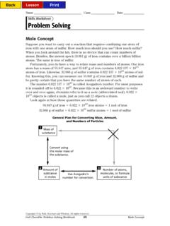
Skills Worksheet Problem Solving - School of Arts & Sciences

Holt ChemFile: Problem-Solving Workbook 49 Mole Concept Name Class Date Problem Solving continued PROBLEMS INVOLVING ATOMS AND ELEMENTS Sample Problem 1 A chemist has a jar containing 388.2 g of iron filings. How many moles of iron does the jar contain? Solution ANALYZE What is given in the problem? mass of iron in grams

  Problem

18.06 Problem Set 7 - Solutions

Problem 5: (10=5+5) (a) If A (an n × n matrix) has n nonnegative eigenvalues λ k and independent eigenvectors x k, and if we define “ √ A” as the matrix with eigenvalues √ λ k and the same eigenvectors, show that (√ A)2 = A. Solution We can decompose A into A = SΛS−1, where S is the matrix consists of eigenvectors of A, and Λ = λ

  Problem