
Lecture 9: Hidden Markov Models
t(4) 0.0 0.25 0.0000 0.01562 0.00000 0.00098 0.00049 0.00037 0.00000 0.00000 t(5) 0.0 0.00 0.0625 0.00000 0.00391 0.00000 0.00000 0.00000 0.00009 0.00007 Note that probabilities decrease with the length of the sequence This is due to the fact that we are looking at a joint probability; this phenomenon would not happen for conditional probabilities
Download Lecture 9: Hidden Markov Models

Information
Domain:
Source:
Link to this page:
Documents from same domain

COMP 551 –Applied Machine Learning Lecture 1: Introduction
www.cs.mcgill.ca• Ryan Lowe • Currently pursuing a PhD in the reasoning and learning lab • Ryan’s research interests ... • Hastie, Tibshirani& Friedman. The Elements of Statistical Learning: Data Mining, Inference, and Prediction, 2nd Edition. Springer. 2009.
Introduction to genome biology - cs.mcgill.ca
www.cs.mcgill.caDNA structure • Polynucleotide chains are directional molecules, with slightly different structures marking the two ends of the chains, the so-called 3' end and 5' end. • …

Perspectives on simulation using GPSS - cs.mcgill.ca
www.cs.mcgill.caPerspectives on simulation using GPSS Thomas I. Schriber Graduate School of Business Administration The University of Michigan AM Arbor Ml 48109-1234 USA ABSTRACT A broad overview of the simulation modeling language GPSS is ... mainframe GPSS/H (Release 1, 1977; Release 2, 1988) also runs on the IBM PClATl370.
GPSS Process - cs.mcgill.ca
www.cs.mcgill.caT r ansaction Lif e A tr ansaction mo v es through GPSS b loc ks (as f ar as possib le). Inter nally, its str ucture is on e xactly one of the chains. Str ucture: unique Xact ID, current

Computing Machinery and Intelligence A. M. Turing Mind ...
www.cs.mcgill.caCOMPUTING MACHINERY AND INTELLIGENCE 435 Q : I have K at my K1, and no other pieces.You have only K at K6 and R at R1. It is your move.What do you play ? A : (After a pause of 15 seconds) R-R8 mate. The question and answer method seems to be suitable for

SEMPÉ-GOSCINNY Les vacances du Petit Nicolas
www.cs.mcgill.caSEMPÉ-GOSCINNY Les vacances du Petit Nicolas (niveau A2/B1) Chapitre 2 - La plage, c’est chouette Le père de Nicolas ayant pris sa décision, il ne restait plus qu’à ranger la maison, mettre les housses, enlever les tapis, décrocher les rideaux, faire …

Modelling and Simulation Concepts
www.cs.mcgill.ca1 Basic concepts In the following, an introduction to the basic concepts of modelling and simulation is given. Figure 1 presents modelling and simulation concepts as introduced by Zeigler [Zei84, ZPK00]. Object is some entity in the Real World. Such an object can exhibit widely varying behaviour depending on the context
Graph Representation Learning
www.cs.mcgill.carepresentation learning have led to new state-of-the-art results in numerous domains, including chemical synthesis, 3D-vision, recommender systems, question answering, ... Chapter 1 Introduction Graphs are a ubiquitous data structure and a universal language for describing complex systems. In the most general view, a graph is simply a collection of
Related documents
Chapter 5: JOINT PROBABILITY DISTRIBUTIONS Part 1 ...
homepage.stat.uiowa.eduGiven random variables Xand Y with joint probability fXY(x;y), the conditional probability distribution of Y given X= xis f Yjx(y) = fXY(x;y) fX(x) for fX(x) >0. The conditional probability can be stated as the joint probability over the marginal probability. Note: we can de ne f Xjy(x) in a similar manner if we are interested in that ...
Notes on Probability
www.maths.qmul.ac.ukHere are the course lecture notes for the course MAS108, Probability I, at Queen ... Joint distributions. Independence. Expectations. Mean, ... In our example, both A and B have probability 4/8=1/2. An event is simple if it consists of just a single outcome, and is compound
Probability, Statistics, and Stochastic Processes
ramanujan.math.trinity.educhapters develop probability theory and introduce the axioms of probability, random variables, and joint distributions. The following two chapters are shorter and of an “introduction to” nature: Chapter 4 on limit theorems and Ch apter 5 on simulation. Statistical inference is treated in Chapter 6, which includes a section on Bayesian v

Topic 7: Random Processes
www.ece.tufts.eduES150 { Harvard SEAS 4. ... † Their joint behavior is completely specifled by the joint distributions for all combinations of their time samples. ... Xn = §1 with probability 1 2 for n even Xn = ¡1=3 and 3 with probabilities 9 10 and 1 10 for n odd † Properties of a WSS process:

Lecture 13 Time Series: Stationarity, AR(p) & MA(q)
www.bauer.uh.edu(4) Forecast. • In this lecture, we go over the statistical theory (stationarity, ... To get asymptotic distributions, we also need a CLT for dependent variables, using the concept of mixing and stationarity. Or we can rely on the martingale CLT. RS –EC2 -Lecture 13 4 • Consider the joint probability distribution of the collection of RVs ...

Lecture 7 Asymptotics of OLS - Bauer College of Business
www.bauer.uh.eduRS – Lecture 7 3 Probability Limit: Convergence in probability • Definition: Convergence in probability Let θbe a constant, ε> 0, and n be the index of the sequence of RV xn.If limn→∞Prob[|xn – θ|> ε] = 0 for any ε> 0, we say that xn converges in probabilityto θ. That is, the probability that the difference between xn and θis larger than any ε>0 goes to zero as n …
13 Introduction to Stationary Distributions
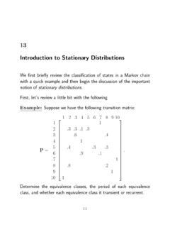
mast.queensu.catransition probability p ijbeside the directed edge between nodes iand jif p ij >0. For example, here is the state transition diagram for the previous example. 4 3 2 6 1 7 10 9 5 8 1 1 1 1 1 0.9 0.1 0.3 0.3 0.4 0.3 0.3 0.1 0.3 0.2 0.8 0.4 0.6 Figure 13.1: State Transition Diagram for Preceding Example Since the diagram displays all one-step ...

Lecture 1: Entropy and mutual information
www.ece.tufts.eduDefinition The mutual information between two continuous random variables X,Y with joint p.d.f f(x,y) is given by I(X;Y) = ZZ f(x,y)log f(x,y) f(x)f(y) dxdy. (26) For two variables it is possible to represent the different entropic quantities with an analogy to set theory. In Figure 4 we see the different quantities, and how the mutual ...
Lecture 4: Kinematic Analysis (Wedge Failure)
www.eoas.ubc.caDiscontinuity Data - Probability Distributions From this, the probability that a given value will be less than dimension x is given by: For example, for a discontinuity set with a mean spacing of 2 m, the probabilities that the spacing will be less than: 1 m 5 m Negative exponential Wyllie & Mah (2004) function:

Multiple Life Models
users.math.msu.eduxy is the probability that at least one of lives (x) and (y) will be alive after tyears. In contrast: t xy q is the probability that at least one of lives (x) and (y) will be dead within tyears. t q xy is the probability that both lives (x) and (y) will be dead within t years. Lecture: Weeks 9-10 (STT 456)Multiple Life ModelsSpring 2015 ...