Multivariate Regression (Chapter 10)

d-

SIAM J. MUMER. ANAL. Vol. 23, No. 5, October 1986 (C) 1986 Society for Industrial andApplied Mathemaics 008 STABLE ATrRACTING SETS IN DYNAMICALSYSTEMS AND IN THEIR ONE-STEP DISCRETIZATIONS*

FINDING RANGE, INTERQUARTILE RANGE, …

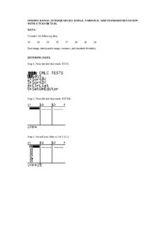
FINDING STANDARD DEVIATION, RANGE AND INTERQUARTILE RANGE. Step 1. When you are done entering data, press STAT and go to CALC. Step 2. Highlight the first option, 1-Var Stats, and press ENTER.

  Ranges, Findings, Deviation, Finding range, Interquartile range, Interquartile

UNIVERSITY OF NEW MEXICO

take University of New Mexico courses while simultaneously attending high school or during the summer between junior and senior years. This is a part-time status and should not be confused with Early Admission. Please refer to page 22 of the

  University, Mexico, University of new mexico

Eigenvalues and Eigenvectors

© 2012 Pearson Education, Inc. Slide 5.1- 10 EIGENVECTORS AND EIGENVALUES ! The scalar λ is an eigenvalue of A if and only if the equation has a nontrivial solution,

  Eigenvalue, Eigenvalues and eigenvectors, Eigenvectors

DETERMINANTS BY ROW AND COLUMN EXPANSION

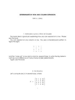
2 TERRY A. LORING 2.1. Expand on the second row (twice). 0 1 4 32 3 1 4 40 6 0 2 32 3 1 6 60 = −3 X0 1 4 32 X3 X1 X4 X4X0 X6 0 2 32

Chapter 4. Gauss-Markov Model - University of New Mexico

Chapter 4, page 4 Result 4.1. b b The BLUE of estimable is uncorrelated with all unbiased estimators of--TT^ zero. Proof: a y First, characterize unbiased estimators of zero as c such that T E( c ) c 0 for all , œ œay aXb bTT or c 0 and , or ( ). Computing the covariance between and weœœ−Xa 0 a X b ayTT TTa -^ have

DEGREE SEQUENCE degree sequence - University of New …

DEGREE SEQUENCE 2 Example 0.1. Up to isomorphism, find all simple graphs with degree sequence (1,1,1,1,2,2,4). Solution: The degree 4 vertex must be adjacent to 0, 1 or 2 of the vertices of degree 2, so we

Lebesgue Measure and The Cantor Set - University of New …

1 Overview De ne a measure. De ne when a set has measure zero. Find the measure of [0;1], I and Q. Construct the Cantor set. Find the measure of the Cantor set.

4.8 Instrumental Variables

What are the consequences of this correlation between x and u? Now higher levels of x have two effects on y. From (4.43) there is both a direct effect via x and an indirect effect via u effecting x which in turn effects y. The goal of regression is to estimate only the rst effect, yielding an estimate of . The OLS

  Correlations, Regression

Covariance, Regression, and Correlation

COVARIANCE, REGRESSION, AND CORRELATION 39 REGRESSION Depending on the causal connections between two variables, xand y, their true relationship may be linear or nonlinear. However, regardless of the true pattern of association, a linear model can always serve as a first approximation. In this case, the analysis is particularly simple, y= fi ...

  Correlations, Regression, Covariance, And correlation

A Simple Explanation of Partial Least Squares

Fact 12. One way to compute the principal components of a matrix X is to perform singular value decomposition, which gives X = UP T; where U is an n nmatrix made up of the eigenvectors of XXT, P is an m mmatrix made up of the eigenvectors of XTX (i.e., the principal components), and is an n mdiagonal matrix made up of the square roots of the non-zero eigenvalues of both XTX and XXT.

  Tesla, Square, Partial, Partial least squares

Correlation and Regression

1 Correlation and Regression Basic terms and concepts 1. A scatter plot is a graphical representation of the relation between two or more variables. In the scatter plot of two variables x and y, each point on the plot is an x-y pair. 2. We use regression and correlation to describe the variation in one or more variables. A. The variation is the sum

  Correlations, Regression, Correlation and regression

Linear Mixed-Effects Regression - Statistics

Nesting typically introduces correlation into data at level-1 Students are level-1 and schools are level-2 Dependence/correlation between students from same school We need to account for this dependence when we model the data. Nathaniel E. Helwig (U of Minnesota) Linear Mixed-Effects Regression Updated 04-Jan-2017 : Slide 8

  Correlations, Regression

Lecture 8a: Spurious Regression

The traditional statistical theory holds when we run regression using (weakly or covariance) stationary variables. For example, when we regress one stationary series onto another stationary series, the coefficient will be close to zero and insignificant if the two series are independent.

  Regression, Covariance

Correlation in Random Variables

Correlation Coefficient The covariance can be normalized to produce what is known as the correlation coefficient, ρ. ρ = cov(X,Y) var(X)var(Y) The correlation coefficient is bounded by −1 ≤ ρ ≤ 1. It will have value ρ = 0 when the covariance is zero and value ρ = ±1 when X and Y are perfectly correlated or anti-correlated. Lecture 11 4

  Correlations, Covariance

Canonical Correlation a Tutorial

In this case, the relation between SNR and correlation is S N = 2 1 2: (17) This relation between correlation and SNR is illustrated in figure 1 (bottom). A Explanations A.1 A note on correlation and covariance matrices In neural network literature, the matrix C xx in equation 3 is often called a corre-lation matrix. This can be a bit ...

  Tional, Correlations, Tutorials, Canonical, Covariance, Cerro, And correlation, Canonical correlation a tutorial, Corre lation

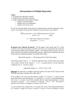
Interpretation in Multiple Regression

estimates (recall the correlation is the covariance divided by the product of the standard deviations, so the covariance is the correlation times the product of the standard deviations. Since the standard deviations are unknown, we use the estimated covariance matrix calculated using the standard errors. In the Results options for Regression, check

  Correlations, Regression, Covariance