
Notes on Probability
Here are the course lecture notes for the course MAS108, Probability I, at Queen ... Joint distributions. Independence. Expectations. Mean, ... In our example, both A and B have probability 4/8=1/2. An event is simple if it consists of just a single outcome, and is compound
Download Notes on Probability

Information
Domain:
Source:
Link to this page:
Documents from same domain
Notes on Combinatorics - QMUL Maths
www.maths.qmul.ac.ukii Preface: What is Combinatorics? Combinatorics, the mathematics of patterns, ..., helps us design com-puter networks, crack security codes, or solve sudokus
Peter J. Cameron October 2013 - QMUL Maths
www.maths.qmul.ac.uk2 Preface Group theory is a central part of modern mathematics. Its origins lie in geome-try (where groups describe in a very detailed way the symmetries of geometric
Solutions to Exercises Chapter 4: Recurrence …
www.maths.qmul.ac.ukSolutions to Exercises Chapter 4: Recurrence relations and generating functions 1 (a) There are n seating positions arranged in a line. Prove that the number
A Course on Number Theory - QMUL Maths
www.maths.qmul.ac.ukiv They will be able to work with Diophantine equations, i.e. polyno-mial equations with integer solutions. They will know some of the famous classical theorems and conjectures in number theory, such as
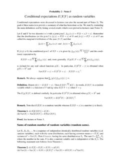
Probability 2 - Notes 5 Conditional expectations E X Y as ...
www.maths.qmul.ac.ukProbability 2 - Notes 5 Conditional expectations E(XjY) as random variables Conditional expectations were discussed in lectures (see also the second part of Notes 3). The
Ten Chapters of the Algebraical Art - QMUL Maths
www.maths.qmul.ac.uk2 CHAPTER 1. WHAT IS MATHEMATICS ABOUT? If and only if We will come back to this later. For now, it means that, for any value of n, either the two statements “n is odd” and “ n2 is odd” are both true, or they are both false.
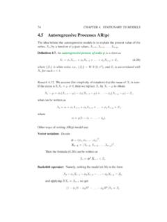
4.5 Autoregressive Processes AR(p)
www.maths.qmul.ac.uk4.5. AUTOREGRESSIVE PROCESSES AR(P) 77 So, we obtained the linear process form of the AR(1) Xt = X∞ j=0 φjZ t−j = X∞ j=0 φ jBZ t. Remark 4.13. Note, that from the equation (4.24) it followsthat ψ(B)is an inverse
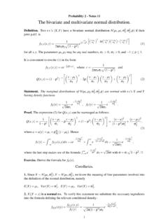
Probability 2 - Notes 11 The bivariate and multivariate ...
www.maths.qmul.ac.ukThis is just the m.g.f. for the multivariate normal distribution with vector of means Am+b and variance-covariance matrix AVAT. Hence, from the uniqueness of the joint m.g.f, Y » N(Am+b;AVAT). Note that from (2) a subset of the Y0s is multivariate normal. NOTE. The results concerning the vector of means and variance-covariance matrix for linear
Notes on Linear Algebra - Queen Mary University of London
www.maths.qmul.ac.ukLinear algebra has two aspects. Abstractly, it is the study of vector spaces over fields, and their linear maps and bilinear forms. Concretely, it is matrix theory: matrices occur in all parts of mathematics and its applications, and everyone work-ing in the mathematical sciences and related areas needs to be able to diagonalise
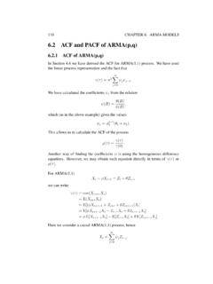
6.2 ACF and PACF of ARMA(p,q)
www.maths.qmul.ac.uk6.2.2 PACF of ARMA(p,q) We have seen earlier that the autocorrelation function of MA(q) models is zero for all lags greater than qas these are q-correlated processes. Hence, the ACF is a good indication of the order of the process. However AR(p) and ARMA(p,q) pro-
Related documents
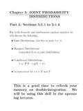
Chapter 5: JOINT PROBABILITY DISTRIBUTIONS Part 1 ...
homepage.stat.uiowa.eduGiven random variables Xand Y with joint probability fXY(x;y), the conditional probability distribution of Y given X= xis f Yjx(y) = fXY(x;y) fX(x) for fX(x) >0. The conditional probability can be stated as the joint probability over the marginal probability. Note: we can de ne f Xjy(x) in a similar manner if we are interested in that ...
Probability, Statistics, and Stochastic Processes
ramanujan.math.trinity.educhapters develop probability theory and introduce the axioms of probability, random variables, and joint distributions. The following two chapters are shorter and of an “introduction to” nature: Chapter 4 on limit theorems and Ch apter 5 on simulation. Statistical inference is treated in Chapter 6, which includes a section on Bayesian v

Topic 7: Random Processes
www.ece.tufts.eduES150 { Harvard SEAS 4. ... † Their joint behavior is completely specifled by the joint distributions for all combinations of their time samples. ... Xn = §1 with probability 1 2 for n even Xn = ¡1=3 and 3 with probabilities 9 10 and 1 10 for n odd † Properties of a WSS process:

Lecture 13 Time Series: Stationarity, AR(p) & MA(q)
www.bauer.uh.edu(4) Forecast. • In this lecture, we go over the statistical theory (stationarity, ... To get asymptotic distributions, we also need a CLT for dependent variables, using the concept of mixing and stationarity. Or we can rely on the martingale CLT. RS –EC2 -Lecture 13 4 • Consider the joint probability distribution of the collection of RVs ...

Lecture 7 Asymptotics of OLS - Bauer College of Business
www.bauer.uh.eduRS – Lecture 7 3 Probability Limit: Convergence in probability • Definition: Convergence in probability Let θbe a constant, ε> 0, and n be the index of the sequence of RV xn.If limn→∞Prob[|xn – θ|> ε] = 0 for any ε> 0, we say that xn converges in probabilityto θ. That is, the probability that the difference between xn and θis larger than any ε>0 goes to zero as n …
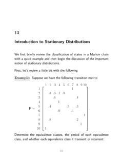
13 Introduction to Stationary Distributions
mast.queensu.catransition probability p ijbeside the directed edge between nodes iand jif p ij >0. For example, here is the state transition diagram for the previous example. 4 3 2 6 1 7 10 9 5 8 1 1 1 1 1 0.9 0.1 0.3 0.3 0.4 0.3 0.3 0.1 0.3 0.2 0.8 0.4 0.6 Figure 13.1: State Transition Diagram for Preceding Example Since the diagram displays all one-step ...

Lecture 1: Entropy and mutual information
www.ece.tufts.eduDefinition The mutual information between two continuous random variables X,Y with joint p.d.f f(x,y) is given by I(X;Y) = ZZ f(x,y)log f(x,y) f(x)f(y) dxdy. (26) For two variables it is possible to represent the different entropic quantities with an analogy to set theory. In Figure 4 we see the different quantities, and how the mutual ...

Lecture 9: Hidden Markov Models
www.cs.mcgill.cat(4) 0.0 0.25 0.0000 0.01562 0.00000 0.00098 0.00049 0.00037 0.00000 0.00000 t(5) 0.0 0.00 0.0625 0.00000 0.00391 0.00000 0.00000 0.00000 0.00009 0.00007 Note that probabilities decrease with the length of the sequence This is due to the fact that we are looking at a joint probability; this phenomenon would not happen for conditional probabilities
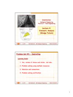
Lecture 4: Kinematic Analysis (Wedge Failure)
www.eoas.ubc.caDiscontinuity Data - Probability Distributions From this, the probability that a given value will be less than dimension x is given by: For example, for a discontinuity set with a mean spacing of 2 m, the probabilities that the spacing will be less than: 1 m 5 m Negative exponential Wyllie & Mah (2004) function:

Multiple Life Models
users.math.msu.eduxy is the probability that at least one of lives (x) and (y) will be alive after tyears. In contrast: t xy q is the probability that at least one of lives (x) and (y) will be dead within tyears. t q xy is the probability that both lives (x) and (y) will be dead within t years. Lecture: Weeks 9-10 (STT 456)Multiple Life ModelsSpring 2015 ...