
Numerical Methods for Engineers
Lecture 1 Binary numbers View this lecture on YouTube We do our arithmetic using decimals, which is a base-ten positional number system. For example, the meaning of the usual decimal notation is illustrated by 524.503 = 5 102 +2 101 +4 100 +5 10 1 +0 10 2 +3 10 3. Each position in a decimal number corresponds to a power of 10.
Download Numerical Methods for Engineers

Information
Domain:
Source:
Link to this page:
Documents from same domain
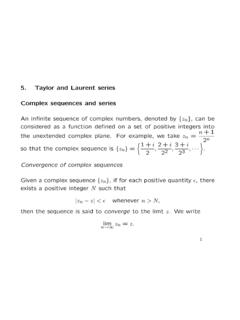
5. Taylor and Laurent series Complex sequences and series
www.math.hkust.edu.hk5. Taylor and Laurent series Complex sequences and series An infinite sequence of complex numbers, denoted by {zn}, can be considered as a function defined on a set of positive integers into the unextended complex plane. For example, we take zn= n+ 1 2n so that the complex sequence is {zn} = ˆ1 + i 2, 2 + i 22, 3 + i 23 ...

Matrix Algebra for Engineers - Hong Kong University of ...
www.math.hkust.edu.hkThe mathematics in this matrix algebra course is at the level of an advanced high school student, but typically students would take this course after completing a university-level single variable calculus course. There are no derivatives and integrals in this course, but student’s are expected to …
Differential Equations - Department of Mathematics, HKUST
www.math.hkust.edu.hkused textbook “Elementary differential equations and boundary value problems” by Boyce & DiPrima (John Wiley & Sons, Inc., Seventh Edition, c 2001). Many of the examples presented in these notes may be found in this book. The material of Chapter 7 is adapted from the textbook “Nonlinear dynamics and chaos” by Steven

Vector Calculus for Engineers - Hong Kong University of ...
www.math.hkust.edu.hkThese are the lecture notes for my online Coursera course,Vector Calculus for Engineers. Students who take this course are expected to already know single-variable differential and integral calculus to the level of an introductory college calculus course. Students should also be familiar with matrices,

Differential Equations for Engineers
www.math.hkust.edu.hkequations 1. By checking all that apply, classify the following differential equation: d3y dx3 +y d2y dx2 = 0 a)first order b)second order c)third order d)ordinary e)partial f)linear g)nonlinear 2. By checking all that apply, classify the following differential equation: 1 x2 d dx x2 dy dx = e y a)first order b)second order c)ordinary d ...
Portfolio Selection Harry Markowitz The Journal of Finance ...
www.math.hkust.edu.hkvary with risk. The hypothesis (or maxim) that the investor does (or should) maximize discounted return must be rejected. If we ignore market im- perfections the foregoing rule never implies that there is a diversified portfolio which is preferable to all non-diversified portfolios. Diversi-

4. Complex integration: Cauchy integral theorem and …
www.math.hkust.edu.hk4. Complex integration: Cauchy integral theorem and Cauchy integral formulas Definite integral of a complex-valued function of a real variable Consider a complex valued function f(t) of a real variable t: f(t) = u(t) + iv(t), which is assumed to be a piecewise continuous function defined in the closed interval a ≤ t ≤ b.
(2.1) Markowitz’s mean-variance formulation (2.2) Two …
www.math.hkust.edu.hkfrontier portfolios need only invest in combinations of these two funds. Remark Any convex combination (that is, weights are non-negative) of ef-ficient portfolios is an efficient portfolio. Let αi ≥ 0 be the weight of Fund i whose rate of return is Ri f. Since E h Ri f i …

Numerical Methods - Hong Kong University of Science and ...
www.math.hkust.edu.hkIn MATLAB, single(224) has the same value as single(224 +1). Since single(224 +1) is exactly halfway between the two consecutive machine numbers 224 and 224 +2, MATLAB rounds to the number with a final zero-bit in f, which is 224. 1.10Machine epsilon Machine epsilon (e mach) is the distance between 1 and the next largest number. If

Systems of Linear Equations - Hong Kong University of ...
www.math.hkust.edu.hkSystems of Linear Equations Beifang Chen 1 Systems of linear equations Linear systems A linear equation in variables x1;x2;:::;xn is an equation of the form a1x1 +a2x2 +¢¢¢+anxn = b; where a1;a2;:::;an and b are constant real or complex numbers. The constant ai is called the coe–cient of xi; and b is called the constant term of the equation. A system of linear equations …
Related documents

6.252 NONLINEAR PROGRAMMING LECTURE 4 …
web.mit.edu6.252 NONLINEAR PROGRAMMING LECTURE 4 CONVERGENCE ANALYSIS OF GRADIENT METHODS LECTURE OUTLINE • Gradient Methods - Choice of Stepsize • Gradient Methods - Convergence Issues

Questions on Assignment 1?
graphics.cs.cmu.edu4 Background Math: Linear Combinations of Vectors • Given two vectors, A and B, walk any distance you like in the A direction, then walk any distance you like in the B direction • The set of all the places (vectors) you can get to this way is the set of linear combinations of A and B. • A set of vectors is said to be linearly independent ...
Lecture notes for Macroeconomics I, 2004 - Yale University
www.econ.yale.eduProof outline. (1) Find a K⁄ candidate; show it is unique. (2) If K0 > K⁄, show that K⁄ < Kt+1 < Kt 8t ‚ 0 (using Kt+1 ¡ Kt = sF (Kt;L) ¡ –Kt).If K0 < K⁄, show that K⁄ > Kt+1 > Kt 8t > 0. (3) We have concluded that Kt is a monotonic sequence, and that it is also bounded. Now use a math theorem: a monotone bounded sequence has a limit. The proof of this theorem establishes not ...
Nonlinear Programming: Concepts, Algorithms and …
cepac.cheme.cmu.eduNonlinear Programming and Process Optimization. 3 Introduction Optimization: given a system or process, find the best solution to this process within constraints. Objective Function: indicator of "goodness" of solution, e.g., cost, yield, profit, etc.
Mathematical Ecnomics
people.tamu.eduLecture Notes 1 Mathematical Ecnomics Guoqiang TIAN Department of Economics Texas A&M University College Station, Texas 77843 (gtian@tamu.edu) This version: August 2018

9.1 Introduction to Integer Programming
www.mcise.uri.edufA nonlinear integer programming problem is an optimization problem in which either the objective function or the left-hand side of some of the constraints are nonlinear functions and some or all of the variables must be integers. Such problems may …
Introduction to Numerical Methods and Matlab …
www.ohiouniversityfaculty.comLecture 30. Euler Methods 122 Lecture 31. Higher Order Methods 126 Lecture 32. Multi-step Methods* 129 Lecture 33. ODE Boundary Value Problems and Finite Di erences 130 Lecture 34. Finite Di erence Method { Nonlinear ODE 134 Lecture 35. Parabolic PDEs - Explicit Method 137 Lecture 36. Solution Instability for the Explicit Method 142 Lecture 37.

Chapter 10 Linear Programming
economics.ubc.ca2 Our second formulation of an LP is: (2) x,x 0 max {x 0: x 0 + c Tx = 0 ; Ax = b ; x ≥ 0 N} where x 0 is a new scalar variable, which is defined by the equality constraint in (2); i.e., x 0 ≡ −c Tx and so minimizing cTx is equivalent to maximizing x 0.It can be seen that the first and second formulations of an LP are completely equivalent. Our third formulation of an LP is the following ...

Introduction to integer programming - MIT OpenCourseWare
ocw.mit.eduGoals of lectures on Integer Programming. Lectures 1 and 2 –Introduce integer programming –Techniques (or tricks) for formulating combinatorial optimization problems as IPs Lectures 3 and 4. –How integer programs are solved (and why they are hard to solve). •Rely on solving LPs fast •Branch and bound and cutting planes Lecture 5.

Quadratic Functions, Optimization, and Quadratic Forms
ocw.mit.edu4 (GP) : minimize f (x) s.t. x ∈ n, where f (x): n → is a function. We often design algorithms for GP by building a local quadratic model of f (·)atagivenpointx =¯x.We form the gradient ∇f (¯x) (the vector of partial derivatives) and the Hessian H(¯x) (the matrix of second partial derivatives), and approximate GP by the following problem which uses the Taylor expansion of f (x)atx ...