NUMERICALSOLUTIONOF ORDINARYDIFFERENTIAL …
11.2 Nonlinear two-point boundary value problems 195 11.2.1 Finite difference methods 197 11.2.2 Shooting methods 201 11.2.3 Collocation methods 204 11.2.4 Other methods and problems 206 Problems 206 12 Volterra integral equations 211 12.1 Solvability theory 212 12.1.1 Special equations 214 12.2 Numerical methods 215 12.2.1 The trapezoidal ...
Download NUMERICALSOLUTIONOF ORDINARYDIFFERENTIAL …

Information
Domain:
Source:
Link to this page:
Documents from same domain
STAT 1030 Business Statistics Additional Final Exam ...
homepage.divms.uiowa.eduSTAT 1030 Business Statistics Additional Final Exam Practice Questions (Part II) Contributed by former TA Scott Wood (also nicknamed "Scooter") 1
Biostatistics 22S:101 Answers to Practice Exam 2
homepage.divms.uiowa.eduBiostatistics 22S:101 Answers to Practice Exam 2 1. A large population contains an unknown proportion (p) of black marbles. A sample of n=200 drawn scientifically

XSL Transformations - University of Iowa
homepage.divms.uiowa.eduXSLT supplies another way to perform these kinds of tasks. XSL (Extensible Stylesheet Language) is an application of XML that provides tools for transforming an XML document
NUMERICALSOLUTIONOF ORDINARYDIFFERENTIAL …
homepage.divms.uiowa.eduNUMERICALSOLUTIONOF ORDINARYDIFFERENTIAL EQUATIONS Kendall Atkinson, Weimin Han, David Stewart ... 3.1 Higher-order differential equations 39 3.2 Numerical methods for systems 42 ... methods for solving boundary value problems of second-order ordinary differential equations. The final chapter, Chapter12, gives an introduct ionto the numerical ...

CHAPTER 3: Random Variables and Probability Distributions
homepage.divms.uiowa.edu1=2 if 4 x < 6 5=6 if 6 x < 10 1 if x 10; nd the probability mass function. Solution: Continuous Probability Distribution: 3.3 A density curve is a curve that is always on or above the horizontal axis, and has area exactly 1 underneath it. A density curve describes the overall pattern of a distribution. The area under the curve and above any

FIXED POINT ITERATION
homepage.divms.uiowa.eduIn general, we are interested in solving the equation x = g(x) by means of xed point iteration: x ... The statement x n+1 ˇg0( )( x n) ... This is an approximation to Newton’s method, with f0(x n) ˇD n. To analyze its convergence, regard it as a xed point iteration with

3.6 Exercises
homepage.divms.uiowa.edu3.6 Exercises 47 (d) Suppose computers are repeatedly selected (assume independence). Find the probability that the 4th selected computer is the first one running Linux. 3.14 A slot machine has 3 wheels. Each wheel has 10 symbols, and each symbol is equally likely when the wheel is spun (assume the wheels act independently of each other). The
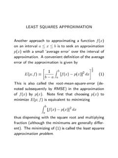
LEAST SQUARES APPROXIMATION - University of Iowa
homepage.divms.uiowa.edugis a quadratic polynomial in the two variables ... ulating this set of conditions leads to a simultaneous linear system. To better understand the form of the linear system, consider the special case of [a,b]=[0,1]. Differenti-ating gwith respect to each ...

A Brief History of Statistics (Selected Topics)
homepage.divms.uiowa.eduthe ancient Greeks – Extended to more than two numbers in the late 1500s in ... milestones in the history of science, and it became a staple in astronomy and other physical sciences by the mid-1800s. • It took until about 1900 before it had fully diffused into other scientific disciplines 11. Some important figures after Laplace and Gauss
Related documents

Solving Differential Equations in R
journal.r-project.orgments three methods to solve boundary value prob-lems. The simplest solution method is the single shooting method, which combines initial value prob-lem integration with a nonlinear root finding algo-rithm (Press et al.,2007). Two more stable solu-tion methods implement a mono implicit Runge-Kutta (MIRK) code, based on the FORTRAN code
Mathematica Tutorial: Advanced Numerical Differential ...
library.wolfram.comIntroduction to Advanced Numerical Differential Equation Solving in Mathematica Overview The Mathematica function NDSolve is a general numerical differential equation solver. It can handle a wide range of ordinary differential equations (ODEs) as well as some partial differential equations (PDEs). In a system of ordinary differential equations there can be any number of
BASKETBALL - Lyons Township High School
www.lths.net2 SHOOTING –Practice the B.E.E.F. method for shooting 3 B = Balance Keep your feet shoulder width apart, with your dominate foot slightly ahead of your non-dominate foot. E = Eyes Focus on the rim. E = Elbow Dominate hand’s elbow should be aligned with your torso in a 90° angle so you are looking at the back of your wrist.

Jeffrey R. Chasnov - Hong Kong University of Science and ...
www.math.hkust.edu.hkis exactly halfway between the two consecutive machine numbers 224 and 224 +2, MATLAB rounds to the number with a final zero-bit in f, which is 2 24 . 1.10Machine epsilon
The Shooting Method for Two-Point Boundary Value …
www.math.usm.eduThe rst method that we will examine is called the shooting method. It treats the two-point boundary value problem as an initial value problem (IVP), in which xplays the role of the time variable, with abeing the \initial time" and bbeing the \ nal time". Speci cally, the shooting method solves the initial value problem y00 = f(x;y;y0); a<x<b;