PARTIAL DIFFERENTIAL EQUATIONS

Real Analysis qual study guide - UC Santa Barbara

Real Analysis qual study guide James C. Hateley 1. Measure Theory Exercise1.1. If AˆR and >0 show 9open sets OˆR such that m(O) m(A) + . Proof: Let fI

  Guide, Analysis, Study, Real, Qual, Real analysis qual study guide

PARTIAL DIFFERENTIAL EQUATIONS - UC Santa Barbara

PARTIAL DIFFERENTIAL EQUATIONS Math 124A { Fall 2010 « Viktor Grigoryan ... 5 Classi cation of second order linear PDEs 21 ... There are a number of properties by which PDEs can be separated into families of similar equations. The two main properties are order and linearity.

  Second, Order, Differential, Equations, Partial, Partial differential equations, Second order

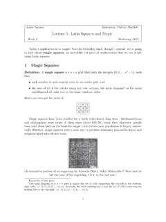
1 Magic Squares - UC Santa Barbara

1 Magic Squares De nition. A magic square is a n n grid lled with the integers f0;1;:::n2 1g, such that each number is used exactly once in our entire grid, and the sum of all of the entries along any row, column, the main diagonal2 or the main antidiagonal all come out to the same constant value. Here’s an example for order 3:

  Square, Magic, 1 magic squares

Finding All the Roots: Sturm’s Theorem

So this process generates a Sturm chain, as claimed. 1.2 Stating and Proving Sturm’s Theorem Sturm chains are pretty odd things; from their construction, it’s not immediately obvious

  Theorem, Sturm, Sturm s theorem, Sturm s theorem sturm

INTERNATIONAL SERIES IN PURE AND APPLIED …

AND APPLIED MATHEMATICS William Ted Martin, E. H. Spanier, G. Springer and P. J. ... Numerical Methods for Scientists and Engineers HILDEBRAND: Introduction to Numerical Analysis ... Applied Mathematics for Engineers and Physicists RALSTON: A First Course in Numerical Analysis

  Methods, Engineer, Scientist, Mathematics, Applied, Applied mathematics, Applied mathematics for engineers

Factoring Cubic Polynomials - UC Santa Barbara

Factoring Cubic Polynomials March 3, 2016 A cubic polynomial is of the form p(x) = a 3x3 + a 2x2 + a 1x+ a 0: The Fundamental Theorem of Algebra guarantees that if a 0;a 1;a 2;a 3 are all real numbers, then we can factor my polynomial into the form

  Polynomials

Practice Problems: Integration by Parts (Solutions)

This is the same as Problem #1, so Z ewsinwdw= 1 2 (ewsinw ewcosw) + C Plug back in w: Z sin(lnx)dx= 1 2 (xsin(lnx) xcos(lnx)) + C 13. R x3 p 1 + x2dx You can do this problem a couple di erent ways. I will show you two solutions. Solution I: You can actually do this problem without using integration by parts. Use the substitution w= 1 + x2 ...

  Practices, Solutions, Part, Problem, Integration, Integration by parts, Practice problems

Practice Problems: Trig Substitution

R x p 1 x4dx Solution: Z x p 1 x4dx= x 1 (x2)2dx Let u= x2, then du= 2xdx: Z x p 1 (x2)2dx= 1 2 Z 1 u2du Now let u= sin , then du= cos d : 1 2 Z p 1 u2du= 1 2 Z 1 sin2 cos d = 1 2 Z cos2 d = 1 4 Z (1+cos2 )d = 1 4 + 1 2 sin2 +C= 1 4 ( +sin cos )+C Plug back in u. Since u= sin , the opposite side will be u, the hypotenuse will be 1, and the

ELEMENTARY DIFFERENTIAL EQUATIONS

Chapter 8 Laplace Transforms 8.1 Introduction to the Laplace Transform 394 8.2 The Inverse Laplace Transform 406 8.3 Solution ofInitial Value Problems 414 8.4 The Unit Step Function 421 8.5 Constant Coefficient Equationswith Piecewise Continuous Forcing Functions 431 8.6 Convolution 441 8.7 Constant Cofficient Equationswith Impulses 453

  Differential, Equations, Elementary, Transform, Elementary differential equations, Laplace transforms, Laplace

ELECTRONICS and CIRCUIT ANALYSIS using MATLAB

Inverse Laplace Transform 6.7 Magnitude and Phase Response of an RLC Circuit CHAPTER SEVEN TWO-PORT NETWORKS EXAMPLE DESCRIPTION 7.1 z-parameters of T-Network 7.2 y-parameters of Pi-Network 7.3 y-parameters of Field Effect Transistor 7.4 h-parameters of Bipolar Junction Transistor 7.5 Transmission Parameters of a Simple Impedance Network 7.6

  Transform, Laplace transforms, Laplace

AnIntroductionto StatisticalSignalProcessing

Laplace argued to the effect that given complete knowledge of the physics of an ... and transform theory and applica-Preface xi tions. Detailed proofs are presented only when within the scope of this background. These simple proofs, however, often provide the groundwork for “handwaving” jus- ... examples, and problems. The

  Example, Transform, Laplace

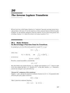
The Inverse Laplace Transform

530 The Inverse Laplace Transform 26.2 Linearity and Using Partial Fractions Linearity of the Inverse Transform The fact that the inverse Laplace transform is linear follows immediately from the linearity of the Laplace transform. To see that, let us consider L−1[αF(s)+βG(s)] where α and β are

  Transform, Inverse, Laplace transforms, Laplace, The inverse laplace transform

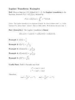
Laplace Transform: Examples - Stanford University

Laplace Transform: Examples Def: Given a function f(t) de ned for t>0. Its Laplace transform is the function, denoted F(s) = Lffg(s), de ned by: F(s) = Lffg(s) = Z 1 0 e stf(t)dt: (Issue: The Laplace transform is an improper integral. So, does it always exist? i.e.: Is the function F(s) always nite?

  Example, Transform, Laplace transforms, Laplace

Laplace Transform solved problems - Univerzita Karlova

Laplace transform for both sides of the given equation. For particular functions we use tables of the Laplace transforms and obtain s(sY(s) y(0)) D(y)(0) = 1 s 1 s2 From this equation we solve Y(s) s3 y(0) + D(y)(0)s2 + s 1 s4 and invert it using the inverse Laplace transform and the same tables again and

  Transform, Laplace transforms, Laplace

SC505 STOCHASTIC PROCESSES Class Notes

SC505 STOCHASTIC PROCESSES Class Notes c Prof. D. Castanon~ & Prof. W. Clem Karl Dept. of Electrical and Computer Engineering Boston University College of Engineering

  Notes, Processes, Class, Stochastic, Sc505 stochastic processes class notes, Sc505

18.03SCF11 text: Delta Functions: Unit Impulse

4. Examples of integration Properties (3) and (2) show that δ(t) is very easy to integrate, as the following examples show: 5 Example 1. 7et2 cos(t)δ(t) dt = 7. All we had to do was evaluate the integrand at t = −5 0. 5 Example 2. 7et2 cos(t)δ(t − 2) dt = 7e4 cos(2). All we had to do was −5 evaluate the integrand at t = 2. 1

  Example

Basics of Signals and Systems - Univr

– Laplace Transform ! Basics – Z-Transform ! Basics Applications in the domain of Bioinformatics 4 . Gloria Menegaz What is a signal? • A signal is a set of information of data ... – Examples: signals defined through a mathematical function or graph • …

  Example, Transform, Laplace transforms, Laplace

Chapter 7: The z-Transform

Convergence of Laplace Transform 7 z-transform is the DTFT of x[n]r n A necessary condition for convergence of the z-transform is the absolute summability of x[n]r n: The range of r for which the z-transform converges is termed the region of convergence (ROC). Convergence example: 1.

  Transform, Laplace transforms, Laplace, The z transform