PARTIAL DIFFERENTIAL EQUATIONS

Real Analysis qual study guide - UC Santa Barbara

Real Analysis qual study guide James C. Hateley 1. Measure Theory Exercise1.1. If AˆR and >0 show 9open sets OˆR such that m(O) m(A) + . Proof: Let fI

  Guide, Analysis, Study, Real, Qual, Real analysis qual study guide

PARTIAL DIFFERENTIAL EQUATIONS - UC Santa Barbara

PARTIAL DIFFERENTIAL EQUATIONS Math 124A { Fall 2010 « Viktor Grigoryan ... 5 Classi cation of second order linear PDEs 21 ... There are a number of properties by which PDEs can be separated into families of similar equations. The two main properties are order and linearity.

  Second, Order, Differential, Equations, Partial, Partial differential equations, Second order

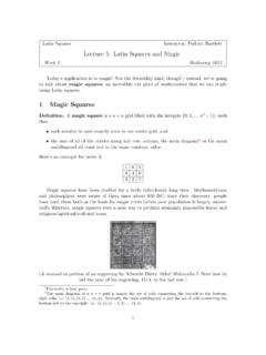
1 Magic Squares - UC Santa Barbara

1 Magic Squares De nition. A magic square is a n n grid lled with the integers f0;1;:::n2 1g, such that each number is used exactly once in our entire grid, and the sum of all of the entries along any row, column, the main diagonal2 or the main antidiagonal all come out to the same constant value. Here’s an example for order 3:

  Square, Magic, 1 magic squares

Finding All the Roots: Sturm’s Theorem

So this process generates a Sturm chain, as claimed. 1.2 Stating and Proving Sturm’s Theorem Sturm chains are pretty odd things; from their construction, it’s not immediately obvious

  Theorem, Sturm, Sturm s theorem, Sturm s theorem sturm

INTERNATIONAL SERIES IN PURE AND APPLIED …

AND APPLIED MATHEMATICS William Ted Martin, E. H. Spanier, G. Springer and P. J. ... Numerical Methods for Scientists and Engineers HILDEBRAND: Introduction to Numerical Analysis ... Applied Mathematics for Engineers and Physicists RALSTON: A First Course in Numerical Analysis

  Methods, Engineer, Scientist, Mathematics, Applied, Applied mathematics, Applied mathematics for engineers

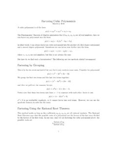
Factoring Cubic Polynomials - UC Santa Barbara

Factoring Cubic Polynomials March 3, 2016 A cubic polynomial is of the form p(x) = a 3x3 + a 2x2 + a 1x+ a 0: The Fundamental Theorem of Algebra guarantees that if a 0;a 1;a 2;a 3 are all real numbers, then we can factor my polynomial into the form

  Polynomials

Practice Problems: Integration by Parts (Solutions)

This is the same as Problem #1, so Z ewsinwdw= 1 2 (ewsinw ewcosw) + C Plug back in w: Z sin(lnx)dx= 1 2 (xsin(lnx) xcos(lnx)) + C 13. R x3 p 1 + x2dx You can do this problem a couple di erent ways. I will show you two solutions. Solution I: You can actually do this problem without using integration by parts. Use the substitution w= 1 + x2 ...

  Practices, Solutions, Part, Problem, Integration, Integration by parts, Practice problems

Practice Problems: Trig Substitution

R x p 1 x4dx Solution: Z x p 1 x4dx= x 1 (x2)2dx Let u= x2, then du= 2xdx: Z x p 1 (x2)2dx= 1 2 Z 1 u2du Now let u= sin , then du= cos d : 1 2 Z p 1 u2du= 1 2 Z 1 sin2 cos d = 1 2 Z cos2 d = 1 4 Z (1+cos2 )d = 1 4 + 1 2 sin2 +C= 1 4 ( +sin cos )+C Plug back in u. Since u= sin , the opposite side will be u, the hypotenuse will be 1, and the

Understanding Poles and Zeros 1 System Poles and Zeros

The transfer function poles are the roots of the characteristic equation, and also the eigenvalues of the system A matrix. The homogeneous response may therefore be written yh(t)= n i=1 Cie pit. (11) The location of the poles in the s-plane therefore define the ncomponents in the homogeneous response as described below: 1.

  Equations, Homogeneous

The Diffusion Equation - Lawrence Berkeley National ...

This equation is known as the heat equation, and it describes the evolution of temperature within a finite, one-dimensional, homogeneous continuum, with no internal sources of heat, subject to some initial and boundary conditions. Indeed, in order to determine uniquely the temperature µ(x;t), we must specify

  Equations, Homogeneous

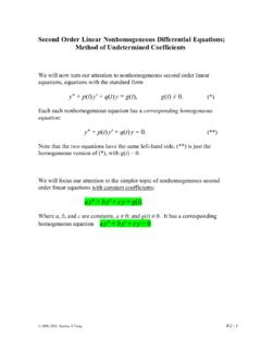
Second Order Linear Nonhomogeneous Differential Equations ...

homogeneous equation (**). Therefore, every solution of (*) can be obtained from a single solution of (*), by adding to it all possible solutions of its corresponding homogeneous equation (**). As a result: Theroem: The general solution of the second order nonhomogeneous linear equation y″ + p(t) y′ + q(t) y = g(t) can be expressed in the ...

  Equations, Homogeneous, Homogeneous equations

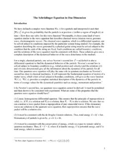
The Schrödinger Equation in One Dimension

Like Newton’s second law, our quantum wave equation cannot be derived. It must be postulated and then shown to be consistent with experiment. What are some of the properties that the quantum wave equation should have? (1) Linear, homogeneous differential equation. This ensures that the principle of superposition is valid, i.e., if Ψ

  Equations, Dimensions, Ingred, Homogeneous, Hsrc, 246 dinger equation in one dimension

Matrices in Computer Graphics - University of Washington

Dec 03, 2001 · Homogeneous Coordinate Transformation Points (x, y, z) in R3 can be identified as a homogeneous vector ( ) →, 1 h z h y h x x y z h with h≠0 on the plane in R4. If we convert a 3D point to a 4D vector, we can represent a transformation to this point with a 4 x 4 matrix. The last coordinate is a scalar term . Graphics

  Homogeneous

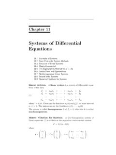
Systems of Differential Equations - University of Utah

corresponding homogeneous system has an equilibrium solution x1(t) = x2(t) = x3(t) = 120. This constant solution is the limit at infinity of the solution to the homogeneous system, using the initial values x1(0) ≈ 162.30, x2(0) ≈119.61, x3(0) ≈78.08. Home Heating Consider a typical home with attic, basement and insulated main floor ...

  Homogeneous

System of First Order Differential Equations

put (3) and (2.2) into the homogeneous equation, we get x0(t) = ‚ve‚t = Ave‚t So Av = ‚v; which indicates that ‚ must be an eigenvalue of A and v is an associate eigenvector. 2.1. A is a 2£2 matrix. Suppose A = • a11 a12 a21 a22 ‚ Then the characteristic polynomial p(‚) of A is p(‚) = jA¡‚Ij = (a11¡‚)⁄(a22 ...

  First, System, Order, Equations, Differential, Homogeneous, System of first order differential equations, Homogeneous equations