Sturm-Liouville Problems

A Brief Review of Elementary Ordinary Differential …

Review of Elementary ODEs 6 Second-Order Linear Homogeneous Equations with Constant Coefficients§ Consider a differential equation of the form ay′′ + by′ + cy = 0 where a, b, and c are (real) constants.

  Review, Differential, Equations, Ordinary, Elementary, Review of elementary ordinary differential

Answers to Selected Exercises - University of Alabama in ...

Answers to Selected Exercises Chapter 1 1. second, fifth, fifth, forty-second 3a i. yes, it is 3a ii. no, it is not 3a iii. no 3b i. no 3b ii. yes 3b iii. no 3c i. yes 3c ii. no 3c iii. no 3d i. no

  Exercise, Answers, Selected, Answers to selected exercises

Reduction of Order - University of Alabama in Huntsville

Reduction of Order for Homogeneous Linear Second-Order Equations 285 Thus, one solution to the above differential equation is y 1(x) = x2. As alreadystated,this method is forfinding a generalsolutionto some homogeneous linear

  Reduction, Second, Order, Differential, Equations, Order equations, Reduction of order

Sturm-Liouville Problems

Sturm-Liouville Problems “Sturm-Liouvilleproblems”areboundary-valueproblemsthat naturallyarisewhen solvingcer-tain partial differential equation problems using a “separation of variables” method that will be discussed in a later chapter. It is the theory behind Sturm-Liouville problems that, …

  Problem, Sturm, Liouville, Sturm liouville problems, Sturm liouvilleproblems, Liouvilleproblems

The Inverse Laplace Transform

The fact that the inverse Laplace transform is linear follows immediately from the linearity of the Laplace transform. To see that, let us consider L−1[αF(s)+βG(s)] where α and β are any two constants and F and G are any two functions for which inverse Laplace transforms

  Transform, Inverse, Laplace, The laplace transform, The inverse laplace transform

Nonlinear Autonomous Systems of Differential Equations

Apr 11, 2014 · Chapter & Page: 43–4 Nonlinear Autonomous Systems of Differential Equations You may have encountered this creature (or its determinant) in other courses involving “two functions of two variables” or “multidimensional change of variables”. It will, in a few pages, provide a link between nonlinear and linear systems.

  System, Equations, Variable, Nonlinear, Two variables

Integration and Differential Equations

the simplest falling object model, starting on page 10). Let us now briefly consider the general case where integration is immediately applicable, and also consider some practical aspects of using both the indefinite integral and the definite integral. ... dy dx = f(x) (2.1)

  Model

Differentiation and the Laplace Transform

We will confirm that this is valid reasoning when we discuss the “inverse Laplace transform” in the next chapter. In general, it is fairly easy to find the Laplace transform of the solution to an initial-value problem involving a linear differential equation with constant coefficients and a ‘reasonable’ forcing function1. Simply take ...

  Transform, Inverse, Laplace transforms, Laplace, The inverse laplace transform

Partial Differential Equations I: Basics and Separable ...

Mar 08, 2014 · Ordinary Differential Equations, Appendex A of these notes. We will be using some of the material discussed there.) 18.1 Intro and Examples Simple Examples If we have a horizontally stretched string vibrating up and down, let u(x,t) = the vertical position at time t of the bit of string at horizontal position x ,

  Differential, Equations, Differential equations

Convolution - University of Alabama in Huntsville

Letusstartwithjustseeingwhat“convolution”is. Afterthat,we’lldiscussusingitwiththe Laplace transform and in solving differential equations. 27.1 Convolution, the Basics Definition and Notation Let f (t) and g(t) be two functions. The convolution of f and g , denoted by f ∗ g , is the function on t ≥ 0 given by f ∗ g(t) = Z t x=0 f ...

  Convolutions, Transform, Laplace transforms, Laplace

Sturm-Liouville Boundary Value Prob- lems

sturm-liouville boundary value problems 109 Types of boundary conditions. We also need to impose the set of homogeneous boundary conditions a1y(a)+ b1y0(a) = 0, a2y(b)+ b2y0(b) = 0.(4.4) The a’s and b’s are constants.For different values, one has special types

  Value, Problem, Boundary, Sturm, Liouville, Prob, Lems, Sturm liouville boundary value prob lems, Sturm liouville boundary value problems

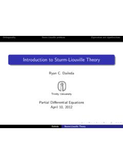
Introduction to Sturm-Liouville Theory

Orthogonality Sturm-Liouville problems Eigenvalues and eigenfunctions Sturm-Liouville equations A Sturm-Liouville equation is a second order linear differential equation that can be written in the form (p(x)y′)′ +(q(x) +λr(x))y = 0. Such an equation is said to be in Sturm-Liouville form. Here p,q and r are specific functions, and λ is a ...

  Sturm, Liouville, Sturm liouville

6 Sturm-Liouville Eigenvalue Problems

Liouville theory. The interested reader can review the literature and more advanced texts for a more in depth analysis. We define the Sturm-Liouville operator as L = d dx p(x) d dx +q(x). (6.2) The Sturm-Liouville eigenvalue problem is given by the differential equation Lu = −λσ(x)u, or d dx p(x) du dx +q(x)u +λσ(x)u = 0, (6.3) for x ...

  Liouville

Chapter 6 Sturm-Liouville Problems - IIT Bombay

Chapter 6 : Sturm-Liouville Problems 55 This has non-trivial solution for the pair (A, B) if and only if fl fl fl fl sin(µπ) 1−cos(µπ)1−cos(µπ) −sin(µπ) fl fl fl fl = 0. (6.14) That is, cos(µπ) = 1.This further implies that µ = ±2n with n ∈ N, and hence λ = 4n2 with n ∈ N. Thus positive eigenvalues are given by

  Chapter, Problem, Chapter 6, Sturm, Liouville, Chapter 6 sturm liouville problems, Sturm liouville problems

1 Solutions in cylindrical coordinates: Bessel functions

To see that this equation is of Sturm-Liouville form, divide through by ρ: ∂ ∂ρ ρ ∂R ∂ρ +k2ρR − m2 ρ R =0 (1) Now we have a Sturm-Liouville equation (slreview notes eqn. 1) with f (ρ)=ρ, g(ρ)=m2/ρ, eigenvalue λ= k2 and weighting function w(ρ)=ρ. Equation (1) is Bessel’s equation. The solutions are orthogonal functions ...

  Liouville

PROPOSED SYLLABUS FOR ‘Mathematical Science'

Sturm-Liouville boundary value problem, Green’s function. Partial Differential Equations (PDEs): Lagrange and Charpit methods for solving first order PDEs, Cauchy problem for first order PDEs. Classification of second order PDEs, General solution of higher order PDEs with constant

  Liouville

Ordinary Differential Equations: Graduate Level Problems ...

Ordinary Differential Equations Igor Yanovsky, 2005 2 Disclaimer: This handbook is intended to assist graduate students with qualifying examination preparation.

Properties of Sturm-Liouville Eigenfunctions and …

Liouville problems. Proposition 6 The set of eigenvalues of a regular Sturm-Liouville problem is countably in nite, and is a monotonically increasing sequence 0 < 1 < 2 < < n< n+1 < with lim n!1 n = 1. The same is true for a periodic Sturm-Liouville problem, except that the sequence is monotonically nondecreasing.

  Properties, Sturm, Liouville, Eigenfunctions, Properties of sturm liouville eigenfunctions and