The Inverse Laplace Transform
532 The Inverse Laplace Transform! Example 26.5: In exercise25.1e on page 523, you found thatthe Laplacetransformof the solution to y′′ + 4y = 20e4t with y(0) = 3 and y′(0) = 12 is Y(s) = 3s2 −28 (s −4). s2 +4 The partial fraction expansion of this is Y(s) = 3s2 −28 (s − 4) s2 +4 A s − + Bs +C s2 +4 for some constants A, B and C .
Download The Inverse Laplace Transform

Information
Domain:
Source:
Link to this page:
Documents from same domain

A Brief Review of Elementary Ordinary Differential …
howellkb.uah.eduReview of Elementary ODEs 6 Second-Order Linear Homogeneous Equations with Constant Coefficients§ Consider a differential equation of the form ay′′ + by′ + cy = 0 where a, b, and c are (real) constants.
Answers to Selected Exercises - University of Alabama in ...
howellkb.uah.eduAnswers to Selected Exercises Chapter 1 1. second, fifth, fifth, forty-second 3a i. yes, it is 3a ii. no, it is not 3a iii. no 3b i. no 3b ii. yes 3b iii. no 3c i. yes 3c ii. no 3c iii. no 3d i. no

Reduction of Order - University of Alabama in Huntsville
howellkb.uah.eduReduction of Order for Homogeneous Linear Second-Order Equations 285 Thus, one solution to the above differential equation is y 1(x) = x2. As alreadystated,this method is forfinding a generalsolutionto some homogeneous linear

Sturm-Liouville Problems
howellkb.uah.eduSturm-Liouville Problems “Sturm-Liouvilleproblems”areboundary-valueproblemsthat naturallyarisewhen solvingcer-tain partial differential equation problems using a “separation of variables” method that will be discussed in a later chapter. It is the theory behind Sturm-Liouville problems that, …

Nonlinear Autonomous Systems of Differential Equations
howellkb.uah.eduApr 11, 2014 · Chapter & Page: 43–4 Nonlinear Autonomous Systems of Differential Equations You may have encountered this creature (or its determinant) in other courses involving “two functions of two variables” or “multidimensional change of variables”. It will, in a few pages, provide a link between nonlinear and linear systems.

Integration and Differential Equations
howellkb.uah.eduthe simplest falling object model, starting on page 10). Let us now briefly consider the general case where integration is immediately applicable, and also consider some practical aspects of using both the indefinite integral and the definite integral. ... dy dx = f(x) (2.1)
Differentiation and the Laplace Transform
howellkb.uah.eduWe will confirm that this is valid reasoning when we discuss the “inverse Laplace transform” in the next chapter. In general, it is fairly easy to find the Laplace transform of the solution to an initial-value problem involving a linear differential equation with constant coefficients and a ‘reasonable’ forcing function1. Simply take ...

Partial Differential Equations I: Basics and Separable ...
howellkb.uah.eduMar 08, 2014 · Ordinary Differential Equations, Appendex A of these notes. We will be using some of the material discussed there.) 18.1 Intro and Examples Simple Examples If we have a horizontally stretched string vibrating up and down, let u(x,t) = the vertical position at time t of the bit of string at horizontal position x ,

Convolution - University of Alabama in Huntsville
howellkb.uah.eduLetusstartwithjustseeingwhat“convolution”is. Afterthat,we’lldiscussusingitwiththe Laplace transform and in solving differential equations. 27.1 Convolution, the Basics Definition and Notation Let f (t) and g(t) be two functions. The convolution of f and g , denoted by f ∗ g , is the function on t ≥ 0 given by f ∗ g(t) = Z t x=0 f ...

Sturm-Liouville Problems
howellkb.uah.eduIt is the theory behind Sturm-Liouville problems that, ultimately, justifies the “separation of variables” method for these partial differential equation problems. The simplest applications lead to the various Fourier series, and less simple applications lead to generalizations
Related documents
Laplace Transform solved problems - cuni.cz
matematika.cuni.czUsing the Laplace transform nd the solution for the following equation @ @t y(t) = e( 3t) with initial conditions y(0) = 4 Dy(0) = 0 Hint. no hint Solution. We denote Y(s) = L(y)(t) the Laplace transform Y(s) of y(t). We perform the Laplace transform for both sides of the given equation. For particular functions we use tables of the Laplace ...
ELEMENTARY DIFFERENTIAL EQUATIONS
ramanujan.math.trinity.eduChapter 8 Laplace Transforms 8.1 Introduction to the Laplace Transform 394 8.2 The Inverse Laplace Transform 406 8.3 Solution ofInitial Value Problems 414 8.4 The Unit Step Function 421 8.5 Constant Coefficient Equationswith Piecewise Continuous Forcing Functions 431 8.6 Convolution 441 8.7 Constant Cofficient Equationswith Impulses 453
1 Z-Transforms, Their Inverses Transfer or System Functions
web.eecs.umich.eduIf you don’t know what a Laplace transform is, you aren’t missing anything that will help you. The above three properties still hold, but computing X(z) now requires use of: ... Solution: Take the z-transforms of the difference equation and of the input. This yields Y(z) −2z−1Y(z) = z−1X(z)−z−2X(z); X(z) = z z −3

Chapter 13: The Laplace Transform in Circuit Analysis
jazapka.people.ysu.edusolution satisfied the given initial conditions and final behavior. ... Transfer Function: the s-domain ratio of the Laplace transform of the output (response) to the Laplace transform of the input (source) ℒ ℒ Example. Finding the transfer function of an RLC circuit If the voltage is the desired output: ...

Solving Differential Equations Using Simulink
people.uncw.eduJul 01, 2019 · related to the Laplace transform L Z t 0 f(t)dt = 1 s F(s), where F(s) is the Laplace transform of f(t). integrate dx dt, producing x(t). introduction to simulink 3 ... The solution shown in Figure 1.13 had a setting of 1 and that in Figure 1.16 …
TABLE OF INVERSE LAPLACE TRANSFORMS
webster.math.umbc.edufirst- and second-order equations, followed by Chapter 5 (the Laplace transform), Chapter 6 (systems), Chapter 8 (nonlinear equations), and part of Chapter 9 (partial differential equations). I generally spend a couple of days giving a rough overview of the omitted chapters: series solutions (Chapter 4) and difference equations (Chapter 7).
Solution of ODEs using Laplace Transforms - Queen's U
chemeng.queensu.caSolution of ODEs We can continue taking Laplace transforms and generate a catalogue of Laplace domain functions. The final aim is the solution of ordinary differential equations. Example Using Laplace Transform, solve Result

Lecture #7 Lagrange's Equations - MIT OpenCourseWare
ocw.mit.eduLaplace, Legendre (Newton 1643-1727) • Contributions o Calculus of variations ... Example: Work in polar coordinates, then transform to rectangular coordinates, e.g. sin cos ... Existence of constraints complicates the solution of the problem.
Section 7.4: Inverse Laplace Transform - University of Florida
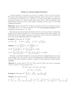
people.clas.ufl.edunding inverse Laplace transforms is a critical step in solving initial value problems. To determine the inverse Laplace transform of a function, we try to match it with the form of an entry in the right-hand column of a Laplace table. Example 1. Determine L 1fFgfor (a) F(s) = 2 s3, (b) F(s) = 3 s 2+ 9, (c) F(s) = s 1 s 2s+ 5. Solution. (a) L 21 ...

Convolution solutions (Sect. 6.6). Convolution of two ...
users.math.msu.eduI Laplace Transform of a convolution. I Impulse response solution. I Solution decomposition theorem. Laplace Transform of a convolution. Theorem (Laplace Transform) If f , g have well-defined Laplace Transforms L[f ], L[g], then L[f ∗ g] = L[f ] L[g]. Proof: The key step is to interchange two integrals. We start we the product of the Laplace ...