Transcription of Lecture10: Expectation-Maximization Algorithm
1 ECE 645: Estimation TheorySpring 2015 Instructor: Prof. Stanley H. ChanLecture 10: Expectation-Maximization Algorithm (LaTeX prepared by Shaobo Fang)May 4, 2015 This lecture note is based on ECE 645 (Spring 2015) by Prof. StanleyH. Chan in the School of Electricaland Computer Engineering at Purdue MotivationConsider a set of data points with their classes labeled, and assume that each class is a Gaussian as shownin Figure 1(a). Given this set of data points, finding the means of twoGaussian can be done easily byestimating the sample mean, as the class labels are imagine that the classes are not labeled as shown in Figure 1(b). How should we determine themean for each of the classes then? In order to solve this problem, we could use an iterative approach: firstmake a guess of the class label for each data point, then compute the means and update the guess of theclass labels again.
2 We repeat until the means problem of estimating parameters in the absence of labels is known as unsupervised learning. Thereare many unsupervised learning methods. We will focus on the Expectation maximization (EM) Algorithm . 10123456 10 8 6 4 202468 Class Labelled Class 1 Class 2 10123456 10 8 6 4 202468 Class UnlabelledFigure 1: Estimation of parameters becomes trivial given the labelledclasses2 The , random variable;y= realization ,xcomplete ,z, missing data. Note thatX= (Y,Z).4. : unknown deterministic parameter. (t):tthestimate of the in the EM (y| ) is the distribution ofYgiven . (X| ) is a random variable taking value off(X| ) (Remember:f( | ) is a function and thus we canput any argument intof( | ) and evaluate its output.) |y, [g(X)] =Rg(x)fX|y, (x|y, )dxis the conditional expectation ofg(X) givenY=yand .8. ( ) = logf(y| ) is the log-likelihood.
3 Note that ( ) depends StepsThe EM- Algorithm consists of two : Givenyand pretending for the moment that (t)is correct, formulate the distribution forthe complete datax:f(x|y, (t)).Then, we calculate the Q-function:Q( | (t))def=EX|y, (t)[logf(X| )]=Zlogf(x| )f(x|y, (t)) : MaximizeQ( | (t)) with regard to : (t+1)= argmax Q( | (t))Properties ofQ( | (t))1. Ideally, if we have the distribution of the complete datax, then finding the parameter can be doneby maximizingf(x| ). However, the complete data is only a virtual thing we created to solved theproblem. In reality we never knowx. All we know is its distributionf(x| ), which depends on whatwe know aboutx. So one way to handle this uncertainty is to compute the average. This average isthe Another way of looking atQ( | (t)). We can treat logf(X| ) as a function of two variablesh(X, ).
4 Maximizing over is problematic because it depends onX. So by taking expectationEX[h(X, )] wecan eliminate the dependency ( | (t)) can be thought of a local approximation of the log-likelihood function ( ): Here, by local we meant thatQ( | (t)) stays close to its previous estimate (t). In fact ifQ( | (t)) Q( (t)| (t)),then ( ) ( (t)).3 Estimating Mean with Partial ObservationLet us consider the first example of the EM Algorithm . Suppose thatwe generated a sequence ofnrandomvariablesYi N( , 2) fori= 1, .. , n. Imagine that we have only observedY= [Y1, Y2, .. , Ym] wherem < n. How should we estimate based onY?Intuitively, the estimated should be the sample mean of themobservationsb =1mPmi=1Yi. However,in this example we would like to derive the EM Algorithm and see if the EM Algorithm would match withour :To start the EM Algorithm , we first need to specify the missing data and the complete data.
5 Inthis problem, the missing data isZ= [Ym+1, .. , Yn], and the complete data isX= [Y,Z]. The distributionofXis:logf(X| ) = n2log(2 2) nXi=1(Yi )22 2.(1)2 Therefore, the Q function isQ( | (t))def=EX|Y, (t)[logf(X| )]=EX|Y, (t)" n2log(2 2) mXi=1(Yi )22 2 nXi=m+1(Yi )22 2#= n2log(2 2) mXi=1(yi )22 2 nXi=m+1EX|Y, (t)[(Yi )2]2 last expectation can be evaluated asEYi|Y, (t)[(Yi )2] =EYi|Y, (t)[Y2i 2Yi + 2]= [( (t))2+ 2 2 (t) + 2].Therefore, the Q function isQ( | (t)) = n2log(2 2) mXi=1(yi )22 2 n m2 2[( (t))2+ 2 2 (t) + 2].In the M-step, we need to maximize the Q-function. To this end, we set Q( | (t)) = 0,which yields that (t+1)=Pmi=1yi+ (n m) (t) is not difficult to show that ast , (t) ( ). Hence, ( )=Pmi=1yin+ 1 mn ( ),which yields ( )=1mmXi= result says that as the EM Algorithm converges, the estimatedparameter converges to the sample meanusing the availablemsamples, which is quite Gaussian Mixture With Known Mean And VarianceOur next example of the EM Algorithm to estimate the mixture weightsof a Gaussian mixture with knownmean and variance.
6 A Gaussian mixture is defined asf(y| ) =kXi=1 iN(y| i, 2i),(2)where = [ 1, .. , k] is called the mixture weight. The mixture weight satisfies the condition thatkXi=1 i= goal is to derive the EM- Algorithm for .3 Solution: We first need to define the missing data. For this problem, we observe that the observed data isY= [y1, y2, , yn]. The missing data can be defined as the label for eachyj, so thatZ= [Z1, Z2, .. , Zn],withZj {1, .. , k}. Consequently, the complete data isX= [X1, X2, , Xn], whereXj= (yj, Zj).The distribution of the complete data can be computed asf(xj| ) =f(yj, zj| ) = zjN(yj| zj, 2zj),Thus, the Q function isQ( | (t)) =EX|,Y, (t){logf(X|, )}=EZ|,y, (t){logf(Z,y|, )}=EZ|,y, (t) lognYj=1 zjN(yj|, zj, 2zj) =nXj=1 EZj|yj, (t)nlog zj+ logN(yj|, zj, 2zj) expectation can be evaluated asEZj|yj, (t){log zj}=Xzjlog zjP(Zj=zj|yj, (t))=kXi=1log iP(Zj=i|yj, (t))|{z}def= (t) summing over allj s, we can further define (t)i=nXj=1 (t)ij=nXj=1P(Zj=i|yj, (t))=nXj=1 (t)iN(yj| i, 2i)Pki=1 (t)iN(yj| i, 2i)Therefore, the Q function becomesQ( | (t)) =nXj=1kXi=1log (t)ij i+C=kXi=1log (t)i i+C,for some constantCindependent of.
7 Maximizing over yields (t+1)= argmax kXi=1 (t)ilog i= (t)iPki=1 (t)i,where the last equality is due to Gibbs inequality. To summarize the EM Algorithm is given in the : Gaussian Mixture with known mean and varianceResult: Estimated fort= 1, do (t)i=nXj=1 (t)iN(yj| i, 2i)Pki=1 (t)iN(yj| i, 2i) (t)i= (t)iPki=1 (t)iendRemark:To solve argmax Pki=1 (t)ilog i, we use the Gibbs inequality. Gibbs inequality states that forall and such thatPni=1 i= 1,Pni=1 i= 1, 0 i 1 and 0 i 1, it holds thatnXi=1 ilog i nXi=1 ilog i,(3)with the equality holds when i= ifor alli. The proof of Gibbs inequality is due to the non-negativity ofthe KL-divergence which we will skip. What we want to show is that if welet i= (t)iPki=1 (t)i, i= i,then the equality holds when: i= (t)iPki=1 (t)i,which is the result we Gaussian MixturePreviously we have been working on Gaussian Mixtures with known mean and variance.
8 However for mostof the time it is likely neither mean nor variance is available for us. Thus,we are interested in deriving anEM- Algorithm that would generally apply for any Gaussian mixture model with only observations that a Gaussian mixture is defined asf(yi| ) =kXi=1 iN(yi| i, i),(4)where def={( i i i)}ki=1is the parameter, withPki=1 i= 1. Our goal is to derive the EM Algorithm forlearning .Solution. We first specify the following data: Observed Data:Y= [Y1, ,Yn] with realizationsy= [y1, ,yn]; Missing Data:Z= [Z1, , Zn] with realizationsz= [z1, , zn], wherezj {1, , k}; Complete Data:X= [X1, ,Xn] with realizationsx= [x1, ,xn] andxj= (yj, zj).Accordingly, the distribution of the complete data isf(yj, zj| ) = zjN(yj| zj, zj)5 Therefore, we can show thatP(Zj=i|yj, (t)) = (t)iN(yj| (t)i, (t)i)Pki=1 (t)iN(yi| (t)i, (t)i).
9 The Q function isQ( , (t)) =EX|y, (t){logf(X| )}=EZ|y, (t){logf(Z,y| )}=EZ|y, (t){log(nYj=1 zjN(yj| zj, zj))}=nXj=1 EZj|yj, (t){log zj 12log| zj| 12(yj zj)T 1zj(yj zj)}+C=nXj=1kXi=1P(Zj=i|yi, (t)){log i 12log| i| 12(yj i)T 1i(yj i)}+C=nXj=1kXi=1 (t)ij{log i 12log| i| 12(yj i)T 1i(yj i)}+C,whereCis a constant independent of .TheMaximizationstep is to solve the following optimization problemmaximize Q( | (t))subject toPki=1 i= 1, i>0, i 0.(5)For i, the maximization ismaximize Pki=1 Pnj=1 (t)ijlog isubject toPki=1 i= 1, i>0(6)The solution of this problem is (t+1)i=Pnj=1 (t)ijPki=1 Pnj=1 (t)ij=Pnj=1 (t)ijn.(7)For i, the maximization can be reduced to solving the equation iQ( | (t)) = 0.(8)The left hand side is iQ( | (t)) = i{nXj=1kXi=1 (t)ij(yj i)T 1i(yj i)}= 1i(nXj=1 (t)ijyj nXj=1 (t)ij i).Therefore, (t+1)i=Pnj=1 (t)ijyiPnj=1 (t)ij(9)6 For i, the maximization is equivalent to solving i( | (t)) = 0.
10 (10)The left hand side is i( | (t)) = 12( nj=1 (t)ij) log| i| i 12nXj=1 (t)ij i{(yj i)T 1i(yj i)}= 12(nXi=1 tij) 1i+12nXj=1 (t)ij 1i(yj i)(yj i)T , t+1i=Pnj=1 (t)ij(yj (t+1)i)(yj (t+1)i)TPni=1 tij.(11)6 Bernoulli MixtureOur next example is to consider a Bernoulli mixture model. To motivatethis problem, let us imagine that wehave a dataset of various items. Our goal is to see whether there isany relationship between the presence orabsence of these items. For example, if the object A ( a tree) was presented, there is some probabilitythat the object B ( a flower) is also presented. However if given certain object C ( a dinosaur)presented it is unlikely to see the object D ( a car, unless you are inJurassic Park!)To setup the problem let us first define some notations. We useY1, ,YNto denoteNimages wehave observed. In each image, there are at mostMitems, so thatYn= [Yn1, , YnM] forn= 1.