Transcription of The lavaan tutorial
1 The lavaan tutorial Yves Rosseel Department of Data Analysis Ghent University (Belgium). July 19, 2021. Abstract If you are new to lavaan , this is the place to start. In this tutorial , we introduce the basic components of lavaan : the model syntax, the fitting functions (cfa, sem and growth), and the main extractor functions (summary, coef, fitted, inspect). After we have provided two simple examples, we briefly discuss some im- portant topics: meanstructures, multiple groups, growth curve models, mediation analysis, and categorical data. Along the way, we hope to give you just enough information to get you started (but no more). Contents 1 Before you start 1. 2 Installation of the package 2. 3 The model syntax 2. 4 A first example: confirmatory factor analysis (CFA) 4. 5 A second example: a structural equation model (SEM) 7. 6 More about the syntax 11. 7 Bringing in the means 14.
2 8 Multiple groups 16. 9 Growth curve models 26. 10 Using categorical variables 28. 11 Using a covariance matrix as input 29. 12 Estimators, standard errors and missing values 31. 13 Indirect effects and mediation analysis 32. 14 Modification Indices 33. 15 Extracting information from a fitted model 34. 16 Multilevel SEM 38. 1 Before you start Before you start, please read these points carefully: First of all, you must have a recent version ( or higher) of R installed. You can download the latest version of R from this page: 1. Some important features are NOT available (yet): full support for hierarchical/multilevel datasets (multilevel cfa, multilevel sem); however version supports two-level cfa/sem with random intercepts only, for continuous complete data support for variable types other than continuous, binary and ordinal (for example: zero-inflated count data, nominal data, non-Gaussian continuous data).
3 Support for discrete latent variables (mixture models, latent classes). We hope to add these features to lavaan in the near future (but please do not ask when). The lavaan package is free open-source software. this means (among other things) that there is no warranty whatsoever. On the other hand, you can verify the source code yourself: https://github. com/yrosseel/ lavaan /. If you need help, you can (only) ask questions in the lavaan discussion group. Go to https://groups. and join the group. Once you have joined the group, you can email your questions to Please do not email me directly. If you think you have found a bug, or if you have a suggestion for improvement, you can either email me directly, or open an issue on github (see ). If you report a bug, always provide a minimal reproducible example (a short R script and some data). 2 Installation of the package The lavaan package is available on CRAN.
4 Therefore, to install lavaan , simply start up R, and type in the R. console: (" lavaan ", dependencies = TRUE). You can check if the installation was succesful by typing library( lavaan ). this is lavaan lavaan is FREE software! Please report any bugs. A startup message will be displayed showing the version number (always report this in your papers), and a reminder that this is free software. If you see this message, you are ready to start. 3 The model syntax At the heart of the lavaan package is the model syntax'. The model syntax is a description of the model to be estimated. In this section, we briefly explain the elements of the lavaan model syntax. More details are given in the examples that follow. In the R environment, a regression formula has the following form: y ~ x1 + x2 + x3 + x4. In this formula, the tilde ( ~ ) is the regression operator. On the left-hand side of the operator, we have the dependent variable (y), and on the right-hand side, we have the independent variables, separated by the +.
5 Operator. In lavaan , a typical model is simply a set (or system) of regression formulas, where some variables (starting with an f' below) may be latent. For example: y ~ f1 + f2 + x1 + x2. f1 ~ f2 + f3. f2 ~ f3 + x1 + x2. If we have latent variables in any of the regression formulas, we must define' them by listing their (manifest or latent) indicators. We do this by using the special operator =~ , which can be read as is measured by. For example, to define the three latent variabels f1, f2 and f3, we can use something like: f1 =~ y1 + y2 + y3. f2 =~ y4 + y5 + y6. f3 =~ y7 + y8 + y9 + y10. 2. Furthermore, variances and covariances are specified using a double tilde' operator, for example: y1 ~~ y1 # variance y1 ~~ y2 # covariance f1 ~~ f2 # covariance And finally, intercepts for observed and latent variables are simple regression formulas with only an intercept (explicitly denoted by the number 1') as the only predictor: y1 ~ 1.
6 F1 ~ 1. Using these four formula types, a large variety of latent variable models can be described. The current set of formula types is summarized in the table below. formula type operator mnemonic latent variable definition =~ is measured by regression ~ is regressed on (residual) (co)variance ~~ is correlated with intercept ~ 1 intercept A complete lavaan model syntax is simply a combination of these formula types, enclosed between single quotes. For example: myModel <- ' # regressions y1 + y2 ~ f1 + f2 + x1 + x2. f1 ~ f2 + f3. f2 ~ f3 + x1 + x2. # latent variable definitions f1 =~ y1 + y2 + y3. f2 =~ y4 + y5 + y6. f3 =~ y7 + y8 + y9 + y10. # variances and covariances y1 ~~ y1. y1 ~~ y2. f1 ~~ f2. # intercepts y1 ~ 1. f1 ~ 1. '. You can type this syntax interactively at the R prompt, but it is much more convenient to type the whole model syntax first in an external text editor.
7 And when you are done, you can copy/paste it to the R console. If you are using RStudio, open a new R script', and type your model syntax (and all other R commands needed for this session) in the source editor of RStudio. And save your script, so you can reuse it later on. The code piece above will produce a model syntax object, called myModel that can be used later when calling a function that actually estimates this model given a dataset. Note that formulas can be split over multiple lines, and you can use comments (starting with the # character) and blank lines within the single quotes to improve the readability of the model syntax. If your model syntax is rather long, or you need to reuse the model syntax over and over again, you may prefer to store it in a separate text file called, say, this text file should be in a human readable format (not a Word document). Within R, you can then read the model syntax from the file as follows: myModel <- readLines("/ ").
8 The argument of readLines is the full path to the file containing the model syntax. Again, the model syntax object can be used later to fit this model given a dataset. 3. 4 A first example: confirmatory factor analysis (CFA). We start with a simple example of confirmatory factor analysis, using the cfa() function, which is a user- friendly function for fitting CFA models. The lavaan package contains a built-in dataset called HolzingerSwineford1939. See the help page for this dataset by typing ?HolzingerSwineford1939. at the R prompt. this is a classic' dataset that is used in many papers and books on Structural Equation Modeling (SEM), including some manuals of commercial SEM software packages. The data consists of mental ability test scores of seventh- and eighth-grade children from two different schools (Pasteur and Grant-White). In our version of the dataset, only 9 out of the original 26 tests are included.
9 A CFA model that is often proposed for these 9 variables consists of three latent variables (or factors), each with three indicators: a visual factor measured by 3 variables: x1, x2 and x3. a textual factor measured by 3 variables: x4, x5 and x6. a speed factor measured by 3 variables: x7, x8 and x9. The figure below contains a graphical representation of the three-factor model. x1. x2. x3 visual x4. x5 textual x6. x7 speed x8. x9. The corresponding lavaan syntax for specifying this model is as follows: visual =~ x1 + x2 + x3. textual =~ x4 + x5 + x6. speed =~ x7 + x8 + x9. In this example, the model syntax only contains three latent variable definitions'. Each formula has the following format: latent variable =~ indicator1 + indicator2 + indicator3. 4. We call these expressions latent variable definitions because they define how the latent variables are manifested by' a set of observed (or manifest) variables, often called indicators'.
10 Note that the special =~" operator in the middle consists of a sign ( = ) character and a tilde ("~") character next to each other. The reason why this model syntax is so short, is that behind the scenes, the cfa() function will take care of several things. First, by default, the factor loading of the first indicator of a latent variable is fixed to 1, thereby fixing the scale of the latent variable. Second, residual variances are added automatically. And third, all exogenous latent variables are correlated by default. this way, the model syntax can be kept concise. On the other hand, the user remains in control, since all this default' behavior can be overriden and/or switched off. We can enter the model syntax using the single quotes: <- ' visual =~ x1 + x2 + x3. textual =~ x4 + x5 + x6. speed =~ x7 + x8 + x9 '. We can now fit the model as follows: fit <- cfa( , data=HolzingerSwineford1939).