Le modèle linéaire généralisé (logit, probit, ) - Master 2 ...

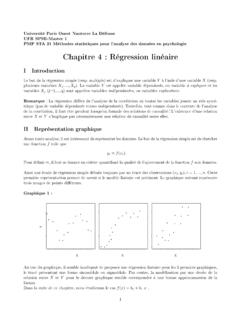
Chapitre 4 : Régression linéaire

fonction linéaire. Graphiquement, la relation est représentée par une droite d'équation y = b0 +b1x. Ce modèle particulier comporte deux paramètres (coe cients) : le coe cient b1: la pente de la droite; b1 > 0 si la droite est croissante, b1 = 0 si la droite est

  Aire, Fonction, Chapitre, Ingresso, Chapitre 4, 233 aire, Fonction lin, 233 gression lin

Chapitre 4 : Régression linéaire

Pour un âge x donné, la tension d'un individu est la somme de deux termes : - 1er terme : b0 + b1x entièrement déterminé par l'âge; - 2ème terme : le terme d'erreur ε qui ariev de façon aléatoire d'un individu à l'autre. Le terme d'erreur ε est une ariablev aléatoire. Elle synthétise toutes les ariablesv in uant sur la tension et qui ne sont pas prises en compte.

Multinomial Logit Models - University of Notre Dame

Mar 06, 2021 · Multinomial Logit Models - Overview Page 1 ... revised March 6, 2021 . This is adapted heavily from Menard’s Applied Logistic Regression analysis; also, Borooah’s Logit and Probit: Ordered and Multinomial Models; Also, Hamilton’s Statistics with Stata, Updated for Version 7. ... (one or two distress incidents), the coefficients tell us ...

  Model, University, Made, Tenor, Logit, Coefficients, Probit, Multinomial, University of notre dame, Probit and logit, Multinomial logit models

Lecture 9: Logit/Probit - Columbia

Logit vs. Probit 0.05.1.15.2-4 -2 0 2 4 Logit Normal The logit function is similar, but has thinner tails than the normal distribution. Logit Function

  Columbia, Logit, Probit

1. Linear Probability Model vs. Logit (or Probit)

Linear Probability Model Logit (probit looks similar) This is the main feature of a logit/probit that distinguishes it from the LPM – predicted probability of =1 is never below 0 or above 1, and the shape is always like the one on the right rather than a straight line.

  Logit, Probit

Lecture 10: Logistical Regression II— Multinomial Data

Logit vs. Probit Review Use with a dichotomous dependent variable Need a link function F(Y) going from the original Y to continuous Y′ Probit: F(Y) = Φ-1(Y) Logit: F(Y) = log[Y/(1-Y)] Do the regression and transform the findings back from Y′to Y, interpreted as a probability

  Logit, Probit

Multinomial Logistic Regression

the ‘exp’ function applied to the coefficients. The Exp(B) is the odds ratio associated with each predictor. We expect predictors which increase the logit to display Exp(B) greater than 1.0, those predictors which do not have an effect on the logit will display an Exp(B) of 1.0 and predictors which decease the logit will have Exp(B)

  Logistics, Regression, Logit, Coefficients, Multinomial, Multinomial logistic regression

R による順序ロジットモデルの推定

logit probit S E E | という関係がある(あくまでもおおよその関係で正確には成り立たない)。ここで E Öprobit はプロビッ トモデルにおける係数の推定値、 EÖlogit はロジットモデルによる係数の推定値である。 練習問題

  Logit, Probit, Logit probit

Mediation Analysiswith Logistic Regression

(estimator=WLSMV), which is a probit analysis and for which standardized coefficients are available (addressing the scaling issue described above). The examples below use negative exchanges (w1neg), depression (w1cesd9), and heart disease (w1hheart) from the LLSSE study (also used in the “Logistic Regression” handout). The hypothesized

  Mediation, Coefficients, Probit

hausman — Hausman specification test - Stata

Test of H0: Difference in coefficients not systematic chi2(3) = (b-B)’[(V_b-V_B)^(-1)](b-B) = 260.40 Prob > chi2 = 0.0000 Under the current specification, our initial hypothesis that the individual-level effects are adequately modeled by a random-effects model is resoundingly rejected. This result is based on the rest of our

  Tests, Specification, Coefficients, Hausman, Hausman hausman specification test

Useful Stata Commands 2019 - Rensselaer Polytechnic Institute

Kenneth L. Simons, 28-Jun-19 1 Useful Stata Commands (for Stata versions 13, 14, & 15) Kenneth L. Simons – This document is updated continually. For the latest version, open it from the course disk space.

  Command, Useful, Stata, Useful stata commands