Transcription of Creating a Random Sample in Excel - Michigan State University
1 Creating a Random Sample in Excel Using your report that contains the complete set of cases: 1. Add row to the right of the Column of numbers you want to Sample and name it whatever you want to call it ( Random Sample ). The example here contains 45 unique visit numbers. 2. In B2 type in the formula =RAND() and then press enter to assign a Random number. 3. Double click on the little box in the lower right corner of the B2 cell. This will repeat the function for all the rows in your report. Make sure there are no blank rows. See Sample on Page 2. 1|Page Creating a Random Sample in Excel 4. Key step replace the function with the value a. Go back to the top of column B and left click to highlight the entire column. b. With column B highlighted do Ctrl+C (or right click and select Copy).
2 C. Click on the bottom portion of Paste to bring up the paste options. Select Paste Values. The numbers won't change, but this step is still necessary. Depending on what version you are working in this option might look different. The key is to copy and select Past Values . This replaces the function with the actual value. If this isn't done, whenever anything changes on the page it will generate a new number. 2|Page Creating a Random Sample in Excel 5. Sort on Column B (named here Random Sample ). a. Highlight all of your data and select Sort from the Data tab. b. Sort by Column B ( Random Sample in this example). It doesn't matter whether the Order is Smallest to Largest or Largest to Smallest. c. Press OK and it will do the sort.
3 After the sort the smallest number comes to the top 6. The rows are now randomized and you can select any grouping of them for your review. In this case the first 15 are selected. You can see that the rows are in Random order by looking at the discharge dates. 3|Pag