Transcription of Lecture 6: Optimization
1 CSC2515: Lecture 6 Optimization1 CSC2515 Fall 2007 Introduction to Machine LearningLecture 6: OptimizationCSC2515: Lecture 6 Optimization2 Regression/Classification & Probabilities The standard setup Assume data are iid from unknown joint distributionor an unknown conditional We see some examplesand we want to infer something about the parameters (weights) of our model The most basic thing is to optimize the parameters using maximum likelihoodor maximum conditional likelihood A better thing to do is maximum penalized (conditional) likelihood, which includes regularization terms such as factorization, shrinkage, input selection, or smoothing An even better thing to do is to go Bayesian, but this is often too computationally demandingp(y,x|w)(y1,x1)(y2,x2)..(yn,xn) p(y|x,w)CSC2515: Lecture 6 Optimization3 Maximum Likelihood Basic ML question: For which setting of the parameters is the data we saw the most likely? Assumes training data are iid, computes the log likelihood, forms a function which depends on the fixed training set we saw and on the argument w:since iidsince Maximizing likelihood is equivalent to minimizing sum squared error, if the noise model is Gaussian and datapoints are iid: (w)=logp(y1,x1,y2,x2.)
2 ,yn,xn|w)=log np(yn,xn|w)= nlogp(yn,xn|w) (w) (w)= 12 2 n(yn f(xn;w))2+constlog = logCSC2515: Lecture 6 Optimization4 Maximum A Posteriori (MAP) MAP asks question: Which setting of the parameters is most likely to be drawn from the prior and then to generate the data from ? It assumes training data are iid, computes the log posterior, and maximizes a function which depends on the fixed training set we saw and on the argument w: , MAP is equivalent to ridge regression, if the noise model is Gaussian, the weight prior is Gaussian, and the datapoints are iid: (w)=logp(w)+logp(y1,x1,y2,x2,..,yn,xn|w) +const=logp(w)+log np(yn,xn|w)=logp(w)+ nlogp(yn,xn|w) (w)p(w)p(X,Y|w) (w)= 12 2 n(yn wTxn)2 iw2i+constCSC2515: Lecture 6 Optimization5 Going Bayesian Ideally we would be Bayesian, applying Bayesrule to compute This is the posterior distributionof the parameters given the data.
3 A true Bayesian would integrate over the posterior to make predictions:but often this is analytically intractable and/or computationally difficult We can settle for maximizing and using the argmaxto make future predictions: this is the maximum a posterior(MAP) approach Many of the penalized maximum likelihood techniques we used for regularization are equivalent to MAP with certain parameter priors: Quadratic weight decay (shrinkage) Gaussian prior Absolute weight decay (lasso) Laplace prior Smoothing on multinomial parameters Dirichlet prior Smoothing on covariance matrices Wishartprior p(ynew|xnew,Y,X)= p(ynew|xnew,w)p(w|Y,X)dwp(w|y1,x1,y2,x2, ..,yn,xn) w CSC2515: Lecture 6 Optimization6 Error Surfaces and Weight Space End result: an error function which we want to minimize can be the negative of the log likelihood or log posterior Consider a fixed training set; think in weight (not input) space.
4 At each setting of the weights there is some error (given the fixed training set): this defines an error surface in weight space. Learning == descending the error surface Notice: if the data are iid, the error function E is a sum of error functions , one per data pointE(w)E(w)EnCSC2515: Lecture 6 Optimization7 Quadratic Error Surfaces and IID Data A very common form for the cost (error) function is the quadratic: This comes up as the log probability when using Gaussians, sinceif the noise model is Gaussian, each of the is an upside-down parabola (a quadratic bowl in higher dimensions). Fact: sum of parabolas (quadratics) is another parabola (quadratic) So the overall error surface is just a quadratic bowl It is easy to find the minimum of a quadratic bowl: For linear regression with Gaussian noise:E(w)=wTAw+2wTb+cEnE(w)=a+bw+cw2 w = b/2cE(w)=a+bTCw w = 12C 1bC=XXTandb= 2 XyTCSC2515: Lecture 6 Optimization8 Partial Derivatives of Error Question: if we wiggle and keep everything else the same,does the error get better or worse?
5 Calculus provides the answer: Plan: use a differentiable cost function and compute partial derivativesof each parameter with respect to this error: Use the chain ruleto compute the derivatives The vector of partial derivatives is called the gradient of the error. The negative gradient points in the direction of steepest error descent in weight space. Three fundamental do we compute the gradient efficiently? we have the gradient, how do we minimize the error? will we end up in weight space? E wk E(w)=( E w1,.., E wM)wkECSC2515: Lecture 6 Optimization9 Steepest Descent Once we have the gradient of the error function, how do we minimize the weights? Steepest descent: If the steps are small enough, then this is guaranteed to converge to at least a local minimum But if we are interested in the rate of convergence, this may not be the best approach Stepsize is a free parameter that has to be chosen carefully for each problem The error surface may be curved differently in different directions.
6 This means that the gradient does not necessarily point directly to the nearest local +1=wt E(w)CSC2515: Lecture 6 Optimization10 Steepest Descent: Far from Ideal CSC2515: Lecture 6 Optimization11 Error Surface: Curvature The local geometry of curvature is measured by the Hessian: the matrix of second-order partial derivatives: Eigenvectors/eigenvalues of the Hessian describe the directions of principal curvature and the amount of curvature in each direction. Maximum sensible stepsize is Rate of convergence depends on2/ max(1 2 min max)Hij= 2E/ wiwjCSC2515: Lecture 6 Optimization12 Adaptive Stepsize No general prescriptions for selecting appropriate learning rate; typically no fixed learning rate appropriate for entire learningperiod Bold driver heuristic: monitor error after each epoch(sweep through entire training set) error decreases, increase learning error increases, decrease rate, reset parameters: Sensible choices for parameters: This is batchgradient descent = =.
7 Wt=wt 1 = , = : Lecture 6 Optimization13 momentum If the error surface is a long and narrow valley, gradient descent goes quickly down the valley walls, but very slowly along the valley floor We can alleviate this problem by updating parameters using a combination of the previous update and the gradient update: Usually is set quite high, about This is like giving momentum to the weights wtj= wt 1+(1 )( E/ wj(wt)) CSC2515: Lecture 6 Optimization14 Convexity, Local Optima Unfortunately, many error functions while differentiable are notunimodal. When using gradient descent we can get stuck in local minima; where we end up depends on where we start. Some very nice error functions ( linear least squares, logistic regression, lasso) are convex, and thus have a unique (global) minimum. Convexity means that the second derivative is always positive. No linear combination of weights can have greater error than thelinear combination of the original errors.
8 But most settings do not lead to convex Optimization : Lecture 6 Optimization15 Mini-Batch and Online Optimization When the dataset is large, computing the exact gradient is expensive This seems wasteful since the only thing we use the gradient for is to compute a small change in the weights, then throw this out and recompute the gradient all over again An approximate gradient is useful as long as it points in roughly the same direction as the true gradient One easy way to do this is to divide the dataset into small batches of examples, compute the gradient using a single batch, make an update, then move to the next batch of examples: mini-batch Optimization In the limit, if each batch contains just one example, then this is the online learning, or stochastic gradient descent mentioned in Lecture 2. These methods are much faster than exact gradient descent, and are very effective when combined with momentum , but care must be taken to ensure convergenceCSC2515: Lecture 6 Optimization16 Line Search Rather than take a fixed step in the direction of the negative gradient or the momentum -smoothed negative gradient, it is possible to do a search along that direction to find the minimumof the function Usually the search is a bisection, which bounds the nearest local minimum along the line between any two points such that there is a third pointw3withE(w3)<E(w1)andE(w3)<E(w2)CSC2 515: Lecture 6 Optimization17 Local Quadratic Approximation By taking a Taylor series of the error function around any pointin weight space, we can make a local quadratic approximationbased on the value, slope, and curvature: Newton s method: jump to the minimum of this quadratic, repeat:w =w H 1(w) E wE(w w0) E(w0)+(w w0)T E w+(w w0)TH(w0)2(w w0)CSC2515.
9 Lecture 6 Optimization18 Second Order Methods Newton s method is an example of a second order optimizationmethod because it makes use of the curvature or Hessian matrix Second order methods often converge much more quickly, but it can be very expensive to calculate and store the Hessian matrix. In general, most people prefer clever first order methods which need only the value of the error function and its gradient with respect to the parameters. Often the sequence of gradients (first order derivatives) can be used to approximatethe second order curvature. This can even be better than the true Hessian, because we can constrain the approximation to always be positive : Lecture 6 Optimization19 Newton and Quasi-Newton Methods Broyden-Fletcher-Goldfarb-Shanno (BFGS); Conjugate-Gradients (CG); Davidon-Fletcher-Powell (DVP); Levenberg-Marquardt (LM) All approximate the Hessian using recent function and gradient evaluations ( , by averaging outer products of gradient vectors, but tracking the ``twist'' in the gradient; by projecting out previous gradient ).
10 Then they use this approximate gradient to come up with a new search direction in which they do a combination of fixed-step, analytic-step and line-search minimizations. Very complex area -- we will go through in detail only the CG method, and a bit of the limited-memory BFGS, CSC2515: Lecture 6 Optimization20 Conjugate Gradients Observation: at the end of a line search, the new gradient is (almost) orthogonal to the direction we just searched in. So if we choose the next search direction to be the new gradient, we will always be searching successively orthogonal directions and things will be very slow. Instead, select a new direction so that, to first order, as we move in the new direction the gradient parallel to the old direction stays zero. This involves blending the current negative gradient with the previous search direction:d(t+1)= g(t+1)+ (t)d(t)CSC2515: Lecture 6 Optimization21 More Conjugate Gradients To first order, all three expressions below satisfy our constraint that along the new search directiongTd(t)=0d(t+1)= g(t+1)+ (t)d(t) (t)=gT(t+1) g(t+1)dT(t) g(t+1)Hestenes Stiefel (t)=gT(t+1) g(t+1)gT(t)g(t)Polak Ribiere (t)=gT(t+1)g(t+1)gT(t)g(t)Fletcher Reeveswhere g(t+1)=g(t+1) g(t)CSC2515: Lecture 6 Optimization22 Conjugate Gradients: ExampleCSC2515: Lecture 6 Optimization23 BFGS One-step memoryless quasi-Newton method A secantmethod iteratively constructing approximation to Hessian matrix Every N steps, where N is number of parameters, search is restarted in the direction of the negative gradientd(t)= g(t)+A(t) w(t)+B(t) g(t)where w(t)=w(t) w(t 1)A(t)= (1+ g(t)T g(t) w(t)T g(t)) w(t)Tg(t) w(t)T g(t)+ g(t)Tg(t) w(t)T g(t)B(t)= w(t)Tg(t) w(t)T g(t)CSC2515.