Gaussian Distribution - Welcome to CEDAR

1 Machine Learning srihari Gaussian Distribution Sargur N. Srihari 1. Machine Learning srihari The Gaussian Distribution Carl Friedrich Gauss For single real-valued variable x 1777-1855. 1 1 2 . N(x | , 2 ) = exp (x ) . (2 ). 2 1/ 2. 2 2. 68% of data lies within of mean 95% within 2 . Parameters: Mean , variance 2, Standard deviation . Precision =1/ 2, E[x]= , Var[x]= 2. For D-dimensional vector x, multivariate Gaussian 1 1 . 1 .. N(x | , ) = exp . (x )T 1. (x ) .. D/2. (2 ) | | 1/2 . 2.. is a mean vector, is a D x D covariance matrix, | | is the determinant of . 2. -1 is also referred to as the precision matrix Machine Learning srihari Covariance Matrix Gives a measure of the dispersion of the data It is a D x D matrix Element in position i,j is the covariance between the ith and jth variables.

2 Covariance between two variables xi and xj is defined as E[(xi- i)(yi- j)]. Can be positive or negative If the variables are independent then the covariance is zero. Then all matrix elements are zero except diagonal elements which represent the variances 3. Machine Learning srihari Importance of Gaussian One variable histogram (uniform over [0,1]). Gaussian arises in many different contexts, , Mean of two variables For a single variable, Gaussian maximizes The two values could be and entropy (for given whose average is More ways of getting mean and variance) than say Sum of set of random Mean of ten variables variables becomes increasingly Gaussian 4.

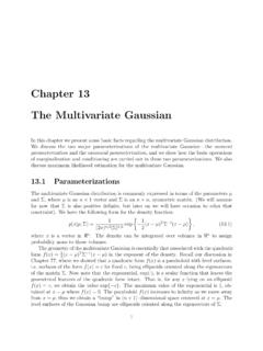
3 Machine Learning srihari Geometry of Gaussian Functional dependence of Two dimensional Gaussian x = (x1,x2). Gaussian on x is through 2 = (x )T 1(x ). Called Mahanalobis Distance reduces to Euclidean distance when is an identity matrix Matrix is symmetric Has an Eigenvector equation ui = iui ui are Eigen vectors Red: Elliptical contour of constant density i are Eigen values Major axes: eigenvectors ui 5. Machine Learning srihari Contours of Constant Density (a) General form Determined by Covariance Matrix Covariances represent how features vary together (b) Diagonal matrix (c) Proportional to (aligned with Identity matrix coordinate axes) (concentric circles).

4 6. Machine Learning srihari Joint Gaussian implies that Marginal and Conditional are Gaussian Joint p(xa, xb). If two sets of variables xa,xb are jointly Gaussian then the two conditional densities and the two marginals are also Gaussian Given joint Gaussian N(x| , ) with = -1 and x = [xa,xb]T where xa are first m components of x and xb are next D-m components Marginal p(xa) and Conditionals Conditional p(xa|xb). p ( x a | x b ) = N ( x | a|b , aa1 ) where a|b = a aa1 ab ( x b b ). Marginals ab . p ( xa ) = N ( xa | a , aa ) where = aa . ba bb 7. Machine Learning srihari If Marginals are Gaussian , Joint need not be Gaussian Constructing such a joint pdf: Consider 2-D Gaussian , zero-mean uncorrelated rvs x and y Due to symmetry about x- and y-axes, we can write marginals: , we only need to integrate over hatched regions Take original 2-D Gaussian and set it to zero over non-hatched quadrants and multiply remaining by 2.

5 We get a 2-D pdf that is definitely NOT Gaussian Machine Learning srihari Maximum Likelihood for the Gaussian Given a data set X=(x1,..xN)T where the observations {xn} are drawn independently Log-likelihood function is given by N. ND N 1. ln p ( X | , ) = ln(2 ) ln | | ( x ) ( x ). n T 1. n 2 2 2 n =1. Derivative wrt is N. ln p ( X | , ) = ( x ). 1. n n =1. N. 1. Whose solution is x ML. =. N n =1. n Maximization is more involved. Yields N. 1. ML =. N. n ML n ML. ( x n =1. ) ( x ) T. 9. Machine Learning srihari Bias of M. L. Estimate of Covariance Matrix For N( , ), of for samples x1,..xN is N.

6 1. ML =. N. (x n =1. n ML )( x n ML )T. arithmetic average of N matrices: (xn ML )(xn ML )T. 1 N. Since E[ ML ] = . N 1 n=1. (xn ML )(xn ML )T. we have E[ ML ] =. N 1. N.. is smaller than the true value of . Thus is biased irrespective of no of samples does not give exact value. For large N inconsequential. Rule of thumb: use 1/N for known mean and 1/(N-1) for estimated mean. Bias does not exist in Bayesian solution. 10. Machine Learning srihari Sequential Estimation In on-line applications and large data sets batch processing of all data points in infeasible Real-time learning scenario where steady stream of data is arriving and predictions must be made before all data is seen Sequential methods allow data points to be processed one-at-a-time and then discarded Sequential learning arises naturally with Bayesian viewpoint for parameters of Gaussian gives a convenient opportunity to discuss more general discussion of sequential estimation for maximum likelihood 11.

7 Machine Learning srihari Sequential Estimation of Gaussian Mean By dissecting contribution of final data point N. 1. ML =. N. x n =1. n 1 N 1. Same as earlier batch result = N -1. ML + ( x N ML ). N. Nice interpretation: After observing N-1 data points we have estimated by MLN-1. We now observe data point xN and we obtain revised estimate by moving old estimate by small amount As N increases contribution from successive points smaller 12. Machine Learning srihari General Sequential Estimation Sequential algorithms cannot always be factored out Robbins and Monro (1951) gave a general solution Consider pair of random variables and z with joint Distribution p(z, ).

8 Conditional expectation of z given is f ( ) = E[ z | ] = zp ( z | )dz Which is called a regression function Same as one that minimizes expected squared loss seen earlier It can be shown that maximum likelihood solution is equivalent to finding the root of the regression function Goal is to find * at which f( *)=0 13. Machine Learning srihari Robbins-Monro Algorithm Defines sequence of successive estimates of root *. as follows ( N ) = ( N 1) + a N 1 z ( ( N 1) ). Where z( (N))is observed value of z when takes the value (N). Coefficients {aN} satisfy reasonable conditions . a a 2. lim a N = 0, N = , N <.

9 N . N =1 N =1. Solution has a form where z involves a derivative of p(x| ) wrt . Special case of Robbons-Monro is solution for Gaussian mean 14. Machine Learning srihari Bayesian Inference for the Gaussian MLE framework gives point estimates for parameters and . Bayesian treatment introduces prior distributions over parameters Case of known variance Likelihood of N observations X={x1,..xN} is N. 1 1 N. 2 . p ( X | ) = p ( xn | ) =. n =1 (2 ). 2 N /2. exp 2. 2 . (x n =1. n ) .. Likelihood function is not a probability Distribution over and is not normalized Note that likelihood function is quadratic in.

10 15. Machine Learning srihari Bayesian formulation for Gaussian mean Likelihood function N. 1 1 N.. p ( X | ) = p ( xn | ) = exp 2 (xn ) . 2. n =1 (2 ). 2 N /2. 2 n =1 . Note that likelihood function is quadratic in . Thus if we choose a prior p( ) which is Gaussian it will be a conjugate Distribution for the likelihood because product of two exponentials will also be a Gaussian p( ) = N( | 0, 02) 16. Machine Learning srihari Bayesian inference: Mean of Gaussian Given Gaussian prior Prior and posterior have same form: conjugacy p( ) = N( | 0, 02). Posterior is given by p( |X) p(X| )p( ). Simplifies to Data points from mean= P( |X) = N( | N, N2) where and known variance= 2 N 02.