Transcription of 6.2 ACF and PACF of ARMA(p,q)
1 110 CHAPTER 6. ARMA MODELS. ACF and PACF of ARMA(p,q). ACF of ARMA(p,q). In Section we have derived the ACF for ARMA(1,1) process. We have used the linear process representation and the fact that . X. 2. ( ) = j j+ . j=0. We have calculated the coefficients j from the relation (B). (B) = , (B). which (as in the above example) gives the values j = j 1. 1 ( 1 + 1 ). This allows us to calculate the ACF of the process ( ). ( ) = . (0). Another way of finding the coefficients is using the homogeneous difference equations. However, we may obtain such equation directly in terms of ( ) or ( ). For ARMA(1,1). Xt Xt 1 = Zt + Zt 1. we can write ( ) = cov(Xt+ , Xt ). = E(Xt+ Xt ). = E[( Xt+ 1 + Zt+ + Zt+ 1 )Xt ]. = E[ Xt+ 1 Xt + Zt+ Xt + Zt+ 1 Xt ]. = E[Xt+ 1 Xt ] + E[Zt+ Xt ] + E[Zt+ 1 Xt ].
2 Here we consider a causal ARMA(1,1) process, hence . X. Xt = j Zt j . j=0. ACF AND PACF OF ARMA(P,Q) 111. This gives . X. E[Zt+ Xt ] = E[Zt+ j Zt j ]. j=0.. X. = j E[Zt+ Zt j ]. j=0. 0 2 for = 0, . =. 0 for 1. Also, . X. E[Zt+ 1 Xt ] = E[Zt+ 1 j Zt j ]. j=0.. X. = j E[Zt+ 1 Zt j ]. j=0.. 1 2 for = 0, = 0 2 for = 1. 0 for 2.. Furthermore, 0 = 1. 1 = + . Putting all these together we obtain ( ) = E[Xt+ 1 Xt ] + E[Zt+ Xt ] + E[Zt+ 1 Xt ].. (1) + 2 (1 + + 2 ) for = 0, = (0) + 2 for = 1, ( 1) for 2.. The ACVF is in fact given here in the form of a homogeneous difference equation of order 1 with initial conditions specifying (0) and (1). Namely, we have ( ) ( 1) = 0 ( ). and the initial conditions are (0) = (1) + 2 (1 + + 2 ).. ( ). (1) = (0) + 2 . Note that the equation ( ).
3 ( ) = ( 1). 112 CHAPTER 6. ARMA MODELS. has an iterative form and we can write (2) = (1). (3) = (2) = 2 (1). (4) = (3) = 3 (1).. ( ) = 1 (1). The polynomial associated with the equation ( ) is 1 z = 0. with root 1. z0 = .. So we can write ( ) = (z0 1 ) 1 (1). This depends only on the root of the associated polynomial and on the initial conditions. Solving ( ) for (0) and (1) we obtain 1 + 2 + 2. (0) = 2. 1 2. and (1 + )( + ). (1) = 2. 1 2. This gives us (1 + )( + ) 1. ( ) = 2 , for 1. 1 2. Finally dividing by (0) we get the ACF, which is the same as the one derived in Section , that is (1 + )( + ) 1. ( ) = , for 1. ( ). 1 + 2 + 2. ACF for ARMA(p,q). Assume that the model (B)Xt = (B)Zt is causal, that is the roots of (B) are outside the unit circle. Then we can write Xt = (B)Zt , ACF AND PACF OF ARMA(P,Q) 113.
4 ACF. x 10. 5. 0. -5. 30 80 130 180 t 0 10 20 30 40 50 . Figure : ARMA(1,1) simulated process xt 1 = zt + 1 , sample ACF and the theoretical ACF of this process. where . X. (B) = j B j j=0. and it follows immediately that E(Xt ) = 0. As in the example for ARMA(1,1), we can obtain a homogeneous differential equation in terms of ( ) with some initial conditions. Namely ( ) = cov(Xt+ , Xt ). " p q ! #. X X. =E j Xt+ j + j Zt+ j Xt j=1 j=0. p q X X. = j E[Xt+ j Xt ] + j E[Zt+ j Xt ]. j=1 j=0. p q X X. = j ( j) + 2 j j . j=1 j= . Here, as before, we used the linear representation of Xt , the fact that Zt+i and Xt are uncorrelated for i > 0 and that i = 0 for i < 0. This gives the general homogeneous difference equation for ( ), ( ) 1 ( 1) .. p ( p) = 0 for max(p, q + 1), ( ).
5 With initial conditions ( ) 1 ( 1) .. p ( p) = 2 ( 0 + +1 1 +..+ q q ) ( ). 114 CHAPTER 6. ARMA MODELS. for 0 < max(p, q + 1). Example ACF of an AR(2) process Let Xt 1 Xt 1 2 Xt 2 = Zt be a causal AR(2) process. From ( ) we have ( ) 1 ( 1) 2 ( 2) = 0 for 2. with initial conditions (. (0) 1 ( 1) 2 ( 2) = 2. (1) 1 (0) 2 ( 1) = 0. It is convenient to write these equations in terms of the autocorrelation function ( ). Dividing them by (0) we obtain .. ( ) 1 ( 1) 2 ( 2) = 0, for 2.. (0) = 1.. ( ). 1. (1) =.. 1 2. We know that a general solution to a second order difference equation is ( ) = c1 z1 + c2 z2 . where z1 and z2 are the roots of the associated polynomial (z) = 1 1 z 2 z 2 , and c1 and c2 can be found from the initial conditions. Take 1 = and 2 = , that is the AR(2) process is Xt 1 + 2 = Zt.)
6 It is a causal process as the coefficients lie in the admissible parameter space. Also, the roots of the associated polynomial (z) = 1 + 2. are z1 = 2 and z2 = 5, , they are outside the unit circle. The initial conditions are . (0) = 1. 7. (1) = =. 1 + 11. ACF AND PACF OF ARMA(P,Q) 115. x ACF. 5. 3. 1. 0. -1. -3. 30 80 130 180 t 0 10 20 30 40 50 . Figure : AR(2) simulated process xt 1 + 2 = zt , sample ACF. and the theoretical ACF of this process. They give the set of equations for c1 and c2 , namely . c1 + c2 = 1. 1 c1 + 1 c2 = 7. 2 5 11. These give 16 5. , c2 = . c1 =. 11 11. and finally we obtain the ACF for this AR(2) process 16 5 24 51 . ( ) = 2 5 = . 11 11 11. Simulated AR(2) process, its sample ACF and the theoretical ACF are shown in Figure As we can see, the theoretical ACF decreases quickly towards zero, but it never attains zero, we say it tails off.
7 116 CHAPTER 6. ARMA MODELS. PACF of ARMA(p,q). We have seen earlier that the autocorrelation function of MA(q) models is zero for all lags greater than q as these are q-correlated processes. Hence, the ACF is a good indication of the order of the process. However AR(p) and ARMA(p,q) pro- cesses are fully correlated, their ACF tails off and never becomes zero, though it may be very close to zero. In such cases it is difficult to identify the process on the ACF basis only. In this section we will consider another correlation function, which together with the ACF will help to identify the models. The function is called Partial Autocor- relation Function (PACF). Before introducing a formal definition of PACF we motivate the idea for AR(1). Let Xt = Xt 1 + Zt be a causal AR(1) process.
8 Then (2) = cov(Xt , Xt 2 ). = cov( Xt 1 + Zt , Xt 2 ). = cov( 2 Xt 2 + Zt 1 + Zt , Xt 2 ). = E[( 2 Xt 2 + Zt 1 + Zt )Xt 2 ]. = 2 (0). The autocorrelation is not zero because Xt depends on Xt 2 through Xt 1 . Due to the iterative kind of AR models there is a chain of dependence. We can break this dependence removing the influence of Xt 1 from both Xt and Xt 2 to obtain Xt Xt 1 and Xt 2 Xt 1. for which the covariance is zero, , cov(Xt Xt 1 , Xt 2 Xt 1 ) = cov(Zt , Xt 2 Xt 1 ) = 0. Similarly, we obtain zero covariance for Xt and Xt 3 after breaking the chain of dependence, removing the dependence of the two variables on Xt 1 and Xt 2 , for Xt f (Xt 1 , Xt 2 ) and Xt 3 f (Xt 1 , Xt 2 ) for some func- tion f . Continuing this we would obtain zero covariances for variables Xt.
9 F (Xt 1 , Xt 2 , .. , Xt +1 ) and Xt f (Xt 1 , Xt 2 , .. , Xt +1 ). Then the only nonzero covariance is for Xt and Xt 1 (nothing in between to break the chain of dependence). These covariances with an appropriate function f divided by the variance of the process are the partial autocorrelations. Hence, for a causal AR(1). process we would have the PACF at lag 1 equal to (1) and at lags > 1 equal to 0. This, together with the tailing off shape of the ACF identifies the process. ACF AND PACF OF ARMA(P,Q) 117. Definition The Partial Autocorrelation Function (PACF) of a zero-mean sta- tionary TS {Xt }t=0,1,.. is defined as 11 = corr(X1 , X0 ) = (1). ( ). = corr(X f( 1) , X0 f( 1) ), 2, where f( 1) = f (X 1 , .. , X1 ). minimizes the mean square linear prediction error E(X f( 1) )2.
10 Remark The subscript at the f function denotes the number of variables the function depends on. Remark By stationarity, is the correlation between variables Xt and Xt . with the linear effect f (Xt 1 , .. , Xt +1 ) = 1 Xt 1 + .. + 1 Xt +1. on each variable removed. Example The PACF of AR(1). Consider a process Xt = Xt 1 + Zt , Zt W N (0, 2 ), where | | < 1, , a causal AR(1). Then by definition 11 = (1) = . To calculate 22 we need to find the function f(1) which is of the form f(1) = X1 . We choose to minimize E(X2 X1 )2 = E(X22 2 X1 X2 + 2 X12 ). = (0) 2 (1) + 2 (0). which is a polynomial in . Taking the derivative with respect to and setting it equal to zero, we obtain 2 (1) + 2 (0) = 0. 118 CHAPTER 6. ARMA MODELS. Hence (1). = = (1) = . (0). and f(1) = X1 . Then 22 = corr(X2 X1 , X0 X1 ) = corr(Z2 , X0 X1 ) = 0.