Transcription of The Usage of Time Series Control Charts for …
1 The Usage of Time Series Control Charts for financial process AnalysisKov k Martin, Kl mek PetrAbstractWe will deal with financial proceedings of the company using methods of SPC (Statistical Proc-ess Control ), specifically through time Series Control Charts . The paper will outline the intersec-tion of two disciplines which are econometrics and statistical process Control . The theoretical part will discuss the methodology of time Series Control Charts and in the research part there will be this methodology demonstrated in three case studies. The first study will focus on the regula-tion of simulated financial flows for a company by CUSUM Control chart . The second study will involve the regulation of financial flows for a heteroskedastic financial process by EWMA con-trol chart . The last case study of our paper will be devoted to applications of ARIMA, EWMA and CUSUM Control Charts in the financial data that are sensitive to the mean shifting while calculating the autocorrelation in the data.
2 In this paper, we highlight the versatility of Control Charts not only in manufacturing but also in managing the financial stability of cash : Statistical process Control , Shewhart s Control Charts , autocorrelation, EWMA Control chart , CU-SUM Control chart , ARIMA Control INTRODUCTIONT raditional SPC schemes can be applied to monitoring the residuals. Subsequent work on this prob-lem can be broadly classified into two themes; those based on time Series models and those which are model-free. For the former, three general approaches have been proposed: those which monitor residuals, those based on direct observations, and those based on new statistics. A brief account of these approaches is presented in this chapter. The time Series model based approach is easy to under-stand and effective in some situations. However, it requires identification of an appropriate time Series model from a set of initial in- Control data. In practice, it may not be easy to establish and may appear to be too complicated to practicing engineers.
3 Hence, the model-free approach has recently attracted much attention. The most popular model-free approach is to form a multivariate statistic from the autocorrelated univariate process , and then monitor it with the corresponding multivariate Control chart . (Krieger et al., 1992) used a multivariate CUSUM scheme. (Apley and Tsung, 2002) adapted the T2 Control chart for monitoring univariate autocorrelated process . (Atienza et al., 1997) proposed a Multivariate boxplot-T2 Control chart . (Dyer et al., 2003) adapted the use of the multivariate EWMA Control chart for autocorrelated processes. Statistical financial flow proceeding means the cash flow management in company. We can avoid possible loss by the cash flow monitoring. This loss can be caused by nondelivery goods, bad financial investment, etc. financial analysis should be done once a year. For our example, we will introduce regulation of simulated financial flows for a company by CUSUM Control chart (see Case Study No 1).
4 In other example, we will describe EWMA Control chart using also monthly values (see Case Study No 2). The end of this paper will be dedicated to the ARIMA, EWMA and CUSUM Control Charts together with some practical example of autocor-related data (see Case Study No 3).Vol. 4, Issue 3, pp. 29-45, September 2012 ISSN 1804-171X (Print), ISSN 1804-1728 (On-line), DOI: of Competitiveness Journal of Competitiveness 02. ElEmENTAR DATA ASSUmPTIONSThis part is mainly focused on crucial problems with the statistical analysis data assumptions. Fundamental assumptions for statistical process regulation can be described as:data normality, symmetry, constant mean of the process ,constant variance (standard deviation) of data,independence, no autocorrelation in data,absence of outliers (Meloun and Militk , 2006).Most data analysis processes and their conclusions are dependent on some fulfilled conditions. If they are not fulfilled all other calculations of means, confidence intervals, quantiles, statistical tests, Shewhart s Charts , capability indices are questionable and not really correct.
5 These calcu-lations usually offer incorrect and inaccurate results and conclusions. Therefore we should be very careful about above mentioned conditions (data normality, symmetry, etc.). Violations of assumptions for the application of regulation by Shewhart s Charts in different technologies are displayed in (Meloun and Militk , 2006).Mentioned conditions should be verified by the help of statistical tests. For example, we can meet data asymmetry by the physical quantities such as strength or viscosity. We can meet strong autocorrelation (dependence) in continuous processes in chemistry, pharmacy, food and metals. Quality of input process material can result into the mean shifting. Not normally distributed data can be seen in ecologic processes very often. Data are very asym-metric with usually lognormal lITERATURE Control Charts CUSUM The CUSUM Control Charts are based on the cumulative sums. They were introduced by Page in 1954.
6 Their main advantage is a very quick detection of relatively small shift in the process mean. This detection is significantly quicker than by the Shewhart s Control Charts . The sequential sums of deviations from 0 are used for the CUSUM Control chart construction. If 0 is a target value for the population mean and if Xj is a sam-ple mean then the CUSUM Control chart is constructed by plotting of variables of the type. This process is called a random walk (Harris and Ross, 1991). CUSUM chart for Individual Values and for Samples Means from Normally Distributed Data Values of xi are independent with the same normal distribution N( , 2) with the known population mean and with the known population standard deviation . We assume logical subgroups with the same volume n. Cumulative sum CUSUM Cn is defined for individual values (n = 1) as: A) on a base of original scale:(1) )(10 ijjiXS njjnxC1)( 1B) on a base of normal distribution where the mean = 0 and the standard deviation = 1: , (2)The CUSUM Cn is almost the same as CUSUM Sn measured in the units of standard deviation.
7 Equation for Cn can be written recurrently (Chandra, 2001): C0 = 0,Cn = Cn 1 + (xn ); and with the same pronciple for Sn: S0 = 0, Sn = Sn 1 + that the original distribution of observed variable N( , 2) changes into N( + , 2) dis-tribution for integer t (at certain moment). It means that the population mean will face a certain shift of . It also means that the shift starts at point (m, Cm) and it grows linearly with the slope . But the population means shift can be more complicated. The CUSUM Control chart can reflect all these changes (Harris and Ross, 1991). CUSUM for Sample Means We have considered mainly the individual values until now. Now, we will consider subgroups with m observations and we calculate the sample means from this subgroups. We have to work with the sample mean standard deviation mx . A shift of mean will not be measured in the units of but in the units of x in this case.
8 We will substitute the individual values of xi with the sample means jx and the process standard deviation with the sample mean standard deviation x in above mentioned formulas. (Lu and Reynolds, 1999)New process Mean Estimate If there is a shift we can estimate a new process mean from the next formula: (3)where N+ and N is a number of selected points from a moment (Chambers and Wheeler, 1992), when Cn+= 0, resp. when Cn- = of CUSUM and Shewhart s Control Charts Fig. 1 Shewhart s Control chart . Source: QC Expert )( jjxU njinUS1jx , , , ,& . SUR& ! +1 & . SUR& +1P Journal of Competitiveness Fig. 2 Control chart CUSUM. Source: QC Expert example shows practically sensitivity of the CUSUM Control chart in comparison with the Shewhart s Control chart for the sample means. The CUSUM Control chart detects process mean deviation towards the lower values (around the subgroup 20 see Figure 1) while the Shewhart s Control chart does not detect this deviation (Harris and Ross, 1991).
9 It does not detect a shift to-wards the upper values (around the subgroup 56). It only detects a big shift around the subgroup 70 (see both Figures 1 and 2) (Lu and Reynolds, 1999). Dynamic Control chart EWMAD ynamic Control Charts EWMA (Exponentially Weighted Moving Average) are used when the following conditions are fulfilled: are not independent, with positive autocorrelationmean is not constant, its changes are slow (Montgomery and Friedman, 1989)A sudden change in mean will only cause a Control limits crossing. These dynamic Charts provide not only the information about in Control process but also about the process dynamic develop-ment. As we mentioned, we consider only data which are not independent with positive autocor-relation. We will explain it now. If the measured observations are influenced by the previous ones we can say that they are dependent. A special case of this dependence is so called autocorrelation of 1st degree when this dependence is linear.
10 If there is a positive autocorrelation in data then the smaller value follows after the smaller value and the higher value follows after the higher value. Data have tendency to preserve their original values. process is not stable in a case of negative autocorrelation. If there is a negative autocorrelation in data then the higher value follows after the smaller value and the smaller value follows after the higher value. Suppose that we measure values x1, x2, x3, .. for the variable X in the process . Parameter (level of forgetting ) is calculated by trying where the function is minimal. Number n is equal to number of measured values of regulated variable. It is recom-mended that n is greater than 50. If the error values of one-step prediction of ek for the optimal value of parameter are not correlated and if they have a normal distribution then the center line CLk, Control limits UCLk and LCLk for the dynamic Control chart EWMA are calculated from the following formulas (Lu and Reynolds, 1999): nkke12 NN &/[ NN S /&/ [X D V NN S 8&/ [X D V Q SNN HQ V where S V is a standard deviation of ek estimate, while ek values are determined for the optimal value of parameter (Yourstone and Montgomery, 1991).]]]