Nonlinear Autonomous Systems of Differential Equations

1 43. Nonlinear Autonomous Systems of Differential Equations Let us now turn our attention to Nonlinear Systems of Differential Equations . We will not attempt to explicitly solve them that is usually just too difficult. Instead, we will see that certain things we learned about the trajectories for linear Systems with constant coefficients can be applied to sketching trajectories for Nonlinear Systems . Consequently, we will be drawing pictures describing the qualitative behavior of the solutions. These pictures can be very informative. Much of the basic theory that we'll develop in the first few sections applies to any suitably differentiable N N Autonomous system of Differential Equations .

2 However, since we are beginners, we will mainly limit ourselves to 2 2 Systems . The Systems of Interest and a Little Review Our interest in this chapter concerns fairly arbitrary 2 2 Autonomous Systems of Differential Equations ; that is, Systems of the form x = f (x, y). , y = g(x, y). which we will often write as x = F(x) with the usual understanding that " # " #. x(t) f (x, y). x = x(t) = and F(x) = . y(t) g(x, y). We will assume that our Autonomous Systems are regular; that is, (as you may recall from chapter 37) we will assume the component functions f and g are continuous and have continuous partial derivatives everywhere on the XY plane.

3 Recall that we discussed trajectories , direction fields , phase planes , critical points and equilibria , and stability for such Systems in chapter 37. Let's refresh our memories with an example: ! Example : Consider the system x = 10x 5x y . ( ). y = 3y + x y 3y 2. 4/11/2014. Chapter & Page: 43 2 Nonlinear Autonomous Systems of Differential Equations To find the critical points, we need to find every ordered pair of real numbers (x, y) at which both x and y are zero. This means algebraically solving the system 0 = 10x 5x y . ( ). 0 = 3y + x y 3y 2. Fortunately, the first equation factors easily: 0 = 10x 5x y = 5x(2 y) , immediately telling us that either x = 0 or y = 2.

4 If x = 0 , then the second equation in system ( ) reduces to 0 = 3y + 0 y 3y 2 = 3y(1 y) , telling us that y = 0 or y = 1 . This gives us two critical points with x = 0 : (0, 0) and (0, 1) . On the other hand, if the first equation in system ( ) holds because y = 2 , then the second equation becomes 0 = 3 2 + x 2 3 22 = 2(x 3) , . implying that x = 3 when y = 2 . This gives us a third critical point, (3, 2) . In summary, our system of Differential Equations has three critical points, (0, 0) , (0, 1) and (3, 2) . No other choices for (x, y) will satisfy algebraic system ( ) (the conditions for a critical point), and any phase portrait for our system of Differential Equations should include these points (remember these points are the trajectories of the constant or equilibrium solutions to the system ).

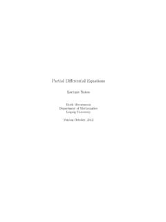
5 A direction field for our system of Differential Equations , along with a few trajectories, has been sketched in figure In that figure, it certainly appears that the critical points (0, 0). and (0, 1) are unstable, and that the critical point (3, 2) is asymptotically stable. In fact, from the trajectories and direction arrows in the regions right around the respective points, it even appears that (0, 0) is an unstable node, (0, 1) is a saddle point, and (3, 2) is an asymptotically stable spiral point. We come back to these observations later. Some more observations: 1.

6 A constant matrix system x = Ax always has (0, 0) as a critical point, and, if A is not degenerate ( , if det(A) 6= 0 ), then (0, 0) is the only critical point. This need not be true for a Nonlinear system . As the above example illustrates, we may have several rather different critical points. And it is quite easy to construct Systems with no critical points (just use x = y 2 + 1 as one of the Equations ). 2. If a constant matrix system x = Ax has an asymptotically stable critical point, then every trajectory in the phase plane converges to that critical point. Again, this need not be the case with a Nonlinear system .

7 In figure , it certainly appears that the critical point (3, 2) is asymptotically stable. However, only those trajectories in the first quadrant appear to converge to this point. Rewriting Systems Using Jacobian Matrices Chapter & Page: 43 3. Y. 4. 3. 2. 1. X. 1 1 2 3 4 5. 1. Figure : A direction field and some trajectories for the system in Example This system has critical points (0, 0) , (0, 1) and (3, 2). The last observation prompts a little more terminology. We will refer to the region containing of all the trajectories that converge to a given asymptotically stable critical point as either the region of asymptotic stability or the basin of attraction for that critical point, and a trajectory bounding that region is called a separatrix for that region.

8 It figure , it appears that the first quadrant is the basin of attraction for critical point (3, 2) , with any trajectory on the positive X axis or Y axis being a separatrix. Rewriting Systems Using Jacobian Matrices The Jacobian Matrix of a system Associated with the regular system x = f (x, y). y = g(x, y). is the Jacobian matrix of the system , also called the Jacobian matrix of f and g with respect to x and y , or the Jacobian matrix of the vector-valued function F = [ f, g]T . This is the matrix-valued function of x and y , normally denoted by either J or ( f,g)/ (x,y) , given by " #.

9 F/ f/. ( f, g) x y J(x, y) = = g/ g/.. (x, y) x y Chapter & Page: 43 4 Nonlinear Autonomous Systems of Differential Equations You may have encountered this creature (or its determinant) in other courses involving two functions of two variables or multidimensional change of variables . It will, in a few pages, provide a link between Nonlinear and linear Systems . ! Example : Let's compute the Jacobian matrix for the system in example , x = 10x 5x y . ( ). y = 3y + x y 3y 2. Here, f (x, y) = 10x 5x y , g(x, y) = 3y + x y 3y 2 , and the Jacobian matrix associated with this system is " #.

10 F/ f/. x y J(x, y) = g/ g/. x y .. [10x 5x y] [10x 5x y] " #. x y 10 5y 5x = .. = . 2. y 3 + x 6y 3y + x y 3y 3y + x y 3y 2. x y In particular, " # " #. 10 5 3 5 1 5 5. J(1, 3) = = . 3 3+1 6 3 3 14. We will be particularly interested in the Jacobian matrices at the critical points found in the previous exercise. So, let's compute them: " # " #. 10 5 0 5 0 10 0. J(0, 0) = = , 0 3+0 6 0 0 3. " # " #. 10 5 1 5 0 5 0. J(0, 1) = =. 1 3 + 0 6(12 ) 0 1 3. and " # " #. 10 5 2 5 3 0 15. J(3, 2) = = . 2 3+3 6 2 2 6. Recollections of Differentiability To see the potential value of a Jacobian matrix, we need to review some basic notions regarding derivatives.