Transcription of MULTIPLE REGRESSION WITH CATEGORICAL DATA
1 ISexMerit PayiSexMerit OF POLITICAL SCIENCEANDINTERNATIONAL RELATIONSPosc/Uapp 816 MULTIPLE REGRESSION WITH CATEGORICAL DATA REGRESSION with CATEGORICAL : Agresti and Finlay Statistical Methods in the Social Sciences, 3rdedition, Chapter 12, pages 449 to INDEPENDENT : what does sex discrimination in employment mean and how can it bemeasured? answer these questions consider these artificial data pertaining to employmentrecords of a sample of employees of Ace : here the dependent variable, Y, is merit pay increase measured in percentand the "independent" variable is sex which is quite obviously a nominal orcategorical goal is to use CATEGORICAL variables to explain variation in Y, a quantitativedependent need to convert the CATEGORICAL variable gender into a form that makessense to REGRESSION way to represent a CATEGORICAL variable is to code the categories 0 and 1 asfollows:Posc/Uapp 816 Class 14 MULTIPLE REGRESSION With CATEGORICAL DataPage 2let X = 1 if sex is "male"0 otherwiseiSexMerit PayiSex Merit Pay (c1) (c2) (c3) (c1) (c2) (c3) : Bob is scored "1" because he is male.
2 Mary is dummy variables, data coded according this 0 and 1 scheme, are in a sensearbitrary but still have some desirable dummy variable, in other words, is a numerical representation of thecategories of a nominal or ordinal : by creating X with scores of 1 and 0 we can transform the abovetable into a set of data that can be analyzed with regular REGRESSION . Here is whatthe data matrix would look like prior to using, say, MINITAB:. for the first column, these data can be considered numeric: merit pay ismeasured in percent, while gender is dummy or binary variable with twovalues, 1 for male and 0 for female. can use these numbers in formulas just like any course, there is something artificial about choosing 0 and 1, for whycouldn t we use 1 and 2 or 33 and or any other pair of numbers? answer is that we could. Using scores of 0 and 1, however, leads toparticularly simple interpretations of the results of REGRESSION analysis, aswe ll see OF the CATEGORICAL variable has K categories ( , region which might have K = 4categories--North, South, Midwest, and West) one uses K - 1 dummy variables asseen regular OLS analysis the parameter estimators can be interpreted as usual: aone-unit change in X leads to $ change in Y.
3 Given the definition of the variables a more straight forward interpretation ispossible. The model is:E(Yi)''$$0%%$$1X1E(Yi)''$$0%%$$1X1''$ $0%%$$1(1)''$$0%%$$1E(Yi)''$$0%%$$1X1''$ $0%%$$1(0)''$$0 Posc/Uapp 816 Class 14 MULTIPLE REGRESSION With CATEGORICAL DataPage model states that the expected value of Y--in this case, the expectedmerit pay increase--equals plus times X. But what are the two0 1possible values of X? consider males; that is, X = 1. Substitute 1 into the expected merit pay increase for males is thus + .0 consider the model for females, , X = 0. Again, make thesubstitution and reduce the can see from these equations that is the expected value of Y0(remember it's merit pay increase in this example) for those subjectsor units coded 0 on X--in this instance it is the expected payincrease of females. Stated differently but equivalently, is the0mean of Y (% pay increase) in the population of units coded 0 on X( , females).1)That is, is where is the mean of the dependent0 0 0variable for the group coded )Remember: the expected value of a random variable is itsmean or E(Y) = iii.
4 Is the "effect," so to speak, of moving or changing from1category 0 to category 1--here of changing from female to male--onthe dependent )Specifically, if > 0, then the expected value of Y is higher1for the group 1 members ( males) than group 0 cases( , females). Thus, if > 0 then men get higher increases1on average than women )On the other hand, if < 0, then group 1 people (units) get1less Y than do group 0 individuals. If < 0, in other words,1 Y'' Ymen'' (1)'' '' 816 Class 14 MULTIPLE REGRESSION With CATEGORICAL DataPage 4 R = .4282 Source df SS MS Fobs_____Regression (sex) 1 Residual 8 Total variation in Y 9 females receive higher pay )If = 0, then both groups have the same expected value , knowing the values of and tells us a lot about the nature of0 1the 0 and 1 to code gender (or any CATEGORICAL variable) thus leads toparticularly simple we used other pairs of numbers, we would get the correct results butthey would be hard to : to put some "flesh" on these concepts suppose we regressed merit pay(Y) on obtain the estimated estimate of the average merit pay increase for women in the populationis percent.
5 (Let X = 0 and simplify the equation.) , on average, get percent more than women. hence their averageincrease "effect" of being male is percent greater merit pay than whatwomen is a partial REGRESSION ANOVA table:Posc/Uapp 816 Class 14 MULTIPLE REGRESSION With CATEGORICAL DataPage the .05 level, the critical value of F with 1 and 8 degrees of freedom Thus, the observed F is barely significant. Since the critical F at level is , the result (the observed "effect" of Y that is) has aprobability of happening by chance of between .05 and . is a problem to consider. A law firm has been asked to represent a group ofwomen who charge that their employer, GANGRENE CHEMICAL CO.,discriminates against them, especially in pay. The women claim that salaryincreases for females are consistently and considerably lower than the raises menreceive. GANGRENE counters that increases are based entirely on jobperformance as measured by an impartial "supervisor rating of work" evaluationwhich includes a number of performance indicators.
6 You have been asked by thelaw firm to make a preliminary assessment of the merits of the claim. To beginwith, you draw a random sample from the company's files:FileQuality $212F901 Production963F204 Production474F801 Production1285F304 Research646F701 Research527F104 Sales738F157 Production199M206 Research12810M803 Sales47411M503 Research34212M702 Sales33013M307 Sales18514M707 Sales33115M401 Sales26716M906 Production51717M508 Production390E(Yi)''$$0%%$$XX%%$$ZZ%%$$W WW''XZ''(Gender) (Workindex)Posc/Uapp 816 Class 14 MULTIPLE REGRESSION With CATEGORICAL DataPage increase is measured in extra dollars per quality of work index ranges from 0 (lowest) to 100 (highest) Division is divisions within the a cursory glance at the data reveal that men get higher increases thanwomen. But the real question is why? for example that men differ from women on other factors such asexperience, division, and job performance evaluations. Are the differencesin salary increases due to these factors?
7 Problem: suppose raises are tied solely to performance ratings. Isthere discrimination in these model:1. X is gender coded: 1 if female 0 otherwise2. Z is job performance evaluation ( , quality of work)3. W = XZ, an interaction term (see below) (W) interaction term has this meaning or interpretation: consider therelationship between Y and Z. So far in this course, this relationship hasbeen measured by , the REGRESSION coefficient of Y on Z. This coefficientZis a partial coefficient in that it measures the impact of Z on Y when othervariables have been held constant. But suppose the effect of Z on Ydepends on the level of another variable, say X. Then, by itself wouldZnot be enough to describe the relationship because there is no simplerelationship between Y and Z. It depends on the level of X. This is the ideaof interaction. be more specific, suppose the relationship between work performance(Z) and pay increase (Y) depends on a worker's sex.
8 That is, suppose aone-unit increase in quality of work performance evaluations for womenbrings a $ increase in salary but a one unit increase in Z brings a $ for men. In this case, the effect of Z, quality of work, depends onor is affected by test this idea we have to create an "interaction" variable by multiplyingZ by X: Y'' Y'' ''W''0(rememberX''0formenandhenceWalsoeq uals0) Y''( )%%( )Z''%% 816 Class 14 MULTIPLE REGRESSION With CATEGORICAL DataPage variable can be added to the model. If it turns out to be non-significantor does not seem to add much to the model's explanatory power, then itcan be dropped. Dropping the interaction term in this context amounts tosaying that the job performance rating has the same impact on salaryincreases for both sexes. If, on the other hand, there is a difference ineffects of Z, the interaction term will explain some of the variation in Y. important point is that W has a substantive meaning. In this context itwould indicate the presence of a second kind of type of discrimination is that on average women get type is that extra increments in job evaluations bring lessrewards for women than OLS estimates of the model is called complete because it contains X, Z, and R for the complete model is.
9 Of the coefficients can be interpreted in the usual way. But using thelogic presented earlier in conjunction with the definition of thedummy variables, there are more straightforward men the estimated equation when Z (job performance) is zero, men can expect on average to geta salary increase of $ For each one-unit increase in their jobevaluations they get an extra $ look at the equation for women X = 1 and hence = and so forth. Workthrough the equations yourself to make sure you grasp what isgoing 816 Class 14 MULTIPLE REGRESSION With CATEGORICAL DataPage 8 Figure 1: Interaction Effect , women can expect an average salary increase of only $ Z is zero and a one-unit increase in the job evaluation index onlybrings an extra 79 cents in figures suggest that there are indeed two types of discriminationworking in the men is $ whereas for women it is $ , a difference0of almost $ men, furthermore, , which measures the return on workZperformance, is $ while for women the return is only $.
10 Is a diagram that illustrates these ideas. (It is not drawn to scale.) FOR estimates are different but since this is a small sample one will want evidencethat the differences are not due to sampling error. We thus need to test thesignificance of . it is not significant we might want to drop it from the would mean that at least one type of discrimination was not strategy is use an extra or added sum of squares the inclusion in a model of a variable or set of variables significantlyincrease the explained sum of squares over what we would expect we will compare two models R' first will be for the model containing all of the variables, amodel we call second is the R for the model without the variables of (Y)''$$0%%$$XX%%$$ZZFobs''(R2com&&R2redu ced)(1&&R2com) (N&&K&&1)gR2comR2reduced1&&R2compR2comp& &R2reducedPosc/Uapp 816 Class 14 MULTIPLE REGRESSION With CATEGORICAL DataPage 9It s called the reduced way to do this is to estimate a complete model as above and obtain anobserved F for it.