Transcription of Quantization of the Free Electromagnetic Field: Photons ...
1 Quantization of the Free Electromagnetic Field: Photons and Operators G. M. Wysin Department of Physics, Kansas State University, Manhattan, KS 66506-2601. August, 2011, Vic osa, Brazil Summary The main ideas and equations for quantized free Electromagnetic fields are developed and summarized here, based on the Quantization procedure for coordinates (components of the vector potential A) and their canonically conjugate momenta (components of the electric field E). Expressions for A, E and magnetic field B are given in terms of the creation and annihilation operators for the fields. Some ideas are proposed for the inter- pretation of Photons at different polarizations: linear and circular. Absorption, emission and stimulated emission are also discussed. 1 Electromagnetic Fields and Quantum Mechanics Here Electromagnetic fields are considered to be quantum objects. It's an interesting subject, and the basis for consideration of interactions of particles with EM fields (light).
2 Quantum theory for light is especially important at low light levels, where the number of light quanta (or Photons ) is small, and the fields cannot be considered to be continuous (opposite of the classical limit, of course!). Here I follow the traditinal approach of Quantization , which is to identify the coordinates and their conjugate momenta. Once that is done, the task is straightforward. Starting from the classical mechanics for Maxwell's equations, the fundamental coordinates and their momenta in the QM sys- tem must have a commutator defined analogous to [x, px ] = ih as in any simple QM system. This gives the correct scale to the quantum fluctuations in the fields and any other dervied quantities. The creation and annihilation operators will have a unit commutator, [a, a ] = 1, but they have to be connected to the fields correctly. I try to show how these relations work. Getting the cor- rect normalization on everything is important when interactions of the EM fields with matter are considered.
3 It is shown that the quantized fields are nothing more than a system of decoupled harmonic oscillators, at a collection of different wavevectors and wave-polarizations. The knowledge of how to quantize simple harmonic oscillators greatly simplifies the EM field problem. In the end, we get to see how the basic quanta of the EM fields, which are called Photons , are created and annihilated in discrete processes of emission and absorption by atoms or matter in general. I also want to discuss different aspects of the Photons , such as their polarization, transition rules, and conservation laws. Later in related notes I'll talk about how this relates to describing two other topics of interest: quantum description of the dielectric response of materials (dielectric function ( )), and, effects involving circularly polarized light incident on a material in the presence of a DC magnetic field (Faraday effect). I want to describe especially the quantum theory for the Faraday effect, which is the rotation of the polarization of linearly polarized light when it passes through a medium in a DC magnetic field parallel to the light rays.
4 That is connected to the dielectric function, hence the interest in these related topics. Maxwell's equations and Lagrangian and Hamiltonian Densities A Lagrangian density for the free EM field is 1 2. E B2.. L= (1). 8 . 1. [It's integral over time and space will give the classical action for a situation with Electromagnetic fields.] This may not be too obvious, but I take it as an excercise for the reader in classical mechanics, because here we want to get to the quantum problem. Maxwell's equations in free space, written for the electric (E) and magnetic (B) fields in CGS units, are 1 B 1 E. B = 0, E+ = 0, E = 0, B =0 (2). c t c t The zero divegence of B and Faraday's Law (1st and 2nd eqns) allow the introduction of vector and scalar potentials, A and , respectively, that give the fields, 1 A. B = A, E = (3). c t I consider a problem far from sources. If sources were present, they would appear in the last two equations in (2), so these same potentials could still apply.
5 The potentials are not unique and have a gauge symmetry. They can be shifted using some guage transformation (f ) without changing the electric and magnetic fields: 1 f A0 = A + f, 0 = (4). c t The Euler-Lagrange variation of the Lagrangian the coordinates q = ( , Ax , Ay , Az ) gives back Maxwell's equations. Recall Euler-Lagrange equation and try it as a practice problem in classical mechanics. To approach Quantization , the canonical momenta pi need to be identified. But there is no time derivative of in L, so there is no p and should be eliminated as a coordinate, in some sense. There are time derivatives of A, hence their canonical momenta are found as . L 1 1 Ai 1. pi = = + = Ei , i = 1, 2, 3 (5). A i 4 c xi c t 4 c The transformation to the Hamiltonian energy density is the Legendre transform, X A 1 2. H= pi q i L = p L = 2 c2 p 2 + ( A) cp (6). i t 8 . When integrated over all space, the last term gives nothing, because E = 0, and the first two terms give a well known result for the effective energy density, in terms of the EM fields, 1.
6 E2 + B2.. H= (7). 8 . We might keep the actual Hamiltonian in terms of the coordinates A and their conjugate momenta p, leading to the classical EM energy, Z . 1 2. H = d3 r 2 c2 p 2 + ( A) (8). 8 . Now it is usual to apply the Coulomb gauge, where = 0 and A = 0. For one, this insures having just three coordinates and their momenta, so the mechanics is consistent. Also that is consistent with the fields needing three coordinates because they are three-dimensional fields. (We don't need six coordinates, because E and B are not independent. In a vague sense, the magnetic and electric fields have some mutual conjugate relationship.) We can use either the Lagrangian or Hamiltonian equations of motion to see the dynamics. For instance, by the Hamiltonian method, we have H H. q i = , p i = (9). pi qi Recall that the variation of a density like this means H H X H H. (10). f f i x i xi f t f t 2. The variation for example coordinate qi = Ax gives the results Ax px 1 2.
7 = 4 c2 px , = Ax (11). t t 4 . By combining these, we see that all the components of the vector potential (and the conjugate momentum, which is proportional to E) satisfy a wave equation, as could be expected! 1 2A. 2 A =0 (12). c2 t2. Wave motion is essentially oscillatory, hence the strong connection of this problem to the harmonic oscillator solutions. The above wave equation has plane wave solutions eik r k t at angular frequency k and wave vector k that have a linear dispersion relation, k = ck. For the total field in some volume V , we can try a Fourier expansion over a collection of these modes, supposing periodic boundary conditions. 1 X. A(r, t) = Ak (t) eik r (13). V k Each coefficient Ak (t) is an amplitude for a wave at the stated wave vector. The different modes are orthogonal (or independent), due to the normalization condition Z. 0. d3 r eik r e ik r = V kk0 (14). The gauge assumption k = 0 then is the same as k Ak = 0, which shows that the waves are transverse.
8 For any k, there are two transverse directions, and hence, two independent polarizations directions, identified by unit vectors ek , = 1, 2. Thus the total amplitude looks like X. Ak = k1 Ak1 + k2 Ak2 = k Ak (15).. Yet, from the wave equation, both polarizations are found to oscillate identically, except perhaps not in phase, Ak (t) = Ak e i k t (16). Now the amplitudes Ak are generally complex, whereas, we want to have the actual field being quantized to be real. This can be accomplished by combining these waves appropriately with their complex conjugates. For example, the simple waves A = cos kx = (eikx + e ikx )/2 and A = sin kx =. (eikx e ikx )/2i are sums of positive and negative wavevectors with particular amplitudes. Try to write A in (13) in a different way that exhibits the positive and negative wavevectors together, 1 X . Ak (t) eik r + A k (t) e ik r . A(r, t) = (17). 2 V k [The sum over k here includes wave vectors in all directions.]
9 Then both k and k are included twice. It is divided by 2 to avoid double counting.] In order for this to be real, a little consideration shows that the 2nd term must be the of the first term, A k = Ak (18). A wave needs to identified by both Ak and its complex conjugate (or equivalently, two real constants). So the vector potential is written in Fourier space as 1 X . Ak (t) eik r + A k (t) e ik r . A(r, t) = (19). 2 V k Note that the reverses the sign on the frequency also, so the first term oscillates at positive frequency and the second at negative frequency. But curiously, both together give a real wave 3. traveling along the direction of k. Based on this expression, the fields are easily determined by applying (3), with ik, i X . k Ak (t) eik r Ak (t) e ik r . E(r, t) = (20). 2c V k i X. k Ak (t) eik r Ak (t) e ik r . B(r, t) = (21). 2 V k Now look at the total energy, , evaluate the Hamiltonian. It should be easy because of the orthogonality of the plane waves, assumed normalized in a box of volume V.
10 We also know that k is perpendicular to A (transverse waves!) which simplifies the magnetic energy. Still, some care is needed in squaring the fields and integrating. There are direct terms (btwn k and itself) and indirect terms (btwn k and k). Z Z. 1 XX h 0 0. i d3 r |E|2 = 2 k k0 d3 r Ak eik r A k e ik r A k0 e ik r Ak0 eik r . (22). 4c V 0. k k Upon integration over the volume, the orthogonality relation will give 2 terms with k0 = k and 2. terms with k0 = k, for 4 equivalent terms in all. The same happens for the calculation of the magnetic energy. Also one can't forget that Ak is the same as A k . These become 1 X k2. Z. 1. d3 r |E|2 = |Ak (t)|2 (23). 8 8 c2. k Z. 1 1 X 2. d3 r |B|2 = k |Ak (t)|2 (24). 8 8 . k Of course, k2 in the expression for magnetic energy is the same as k2 /c2 in that for electric energy. Then it is obvious that the magnetic and electric energies are equal. The net total energy is simple, Z. 1 1 X 2 1 X 2.