Example: dental hygienist
Hilbert spaces - Massachusetts Institute of Technology
70 3. HILBERT SPACES Proof. Take a countable dense subset { which can be arranged as a sequence fv jgand the existence of which is the de nition of separability { and orthonormalize it. Thus if v 1 6= 0 set e i = v 1=kv 1k:Proceeding by induction we can suppose to have found for a given integer nelements e
Information
Domain:
Source:
Link to this page:
Documents from same domain
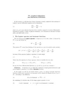
V7. Laplace’s Equation and Harmonic Functions
math.mit.eduA. Existence. Does there exist a φ(x,y) harmonic in some region containing Cand its interior R, and taking on the prescribed boundary values? B. Uniqueness. If it exists, is there only one such φ(x,y)? C. Solving. If there is a unique φ(x,y), determine it by some explicit formula, or approximate it by some numerical method.
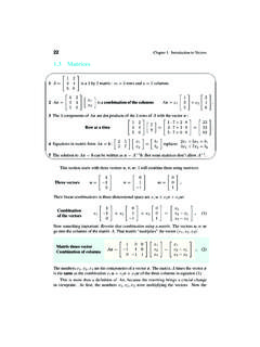
Introduction to Linear Algebra, 5th Edition
math.mit.edu1.3 Matrices 1 A = ... Linear Equations One more change in viewpoint is crucial. Up to now, the numbers x 1,x 2,x 3 were known. The right hand side b was not known. We found that vector of differences by multiplying A times x. Now we think of b as known and we look for x.
Eigenvalues and Eigenvectors
math.mit.eduSpecial properties of a matrix lead to special eigenvalues and eigenvectors. That is a major theme of this chapter (it is captured in a table at the very end). 286 Chapter 6.
Eigenvalues and Eigenvectors - MIT Mathematics
math.mit.edu6.1. Introduction to Eigenvalues 287 Eigenvalues The number is an eigenvalue of Aif and only if I is singular: det.A I/ D 0: (3) This “characteristic equation” det.A I/ D 0 involves only , not x. When A is n by n,
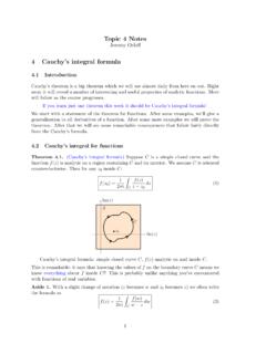
4 Cauchy’s integral formula - MIT Mathematics
math.mit.edu4 Cauchy’s integral formula 4.1 Introduction ... 4 CAUCHY’S INTEGRAL FORMULA 4 4.3.1 Another approach to some basic examples Suppose Cis a simple closed curve around 0. We have seen that Z C 1 z ... Since an integral is basically a sum, this translates to the triangle inequality for integrals.
A FRIENDLY INTRODUCTION TO GROUP THEORY
math.mit.eduA FRIENDLY INTRODUCTION TO GROUP THEORY 3 A good way to check your understanding of the above de nitions is to make sure you understand why the following equation is correct: jhgij= o(g): (1) De nition 5: A group Gis called abelian (or commutative) if gh = hg for all g;h2G. A group is called cyclic if it is generated by a single element, that is,
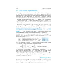
4.3 Least Squares Approximations
math.mit.edu4.3. Least Squares Approximations 221 Figure 4.7: The projection p DAbx is closest to b,sobxminimizes E Dkb Axk2. In this section the situation is just the opposite. There are no solutions to Ax Db. Instead of splitting up x we are splitting up b. Figure 4.3 shows the big picture for least squares. Instead of Ax Db we solve Abx Dp.

Linear programming 1 Basics - MIT Mathematics
math.mit.edu2 subject to: 5x 1 + 7x 2 8 4x 1 + 2x 2 15 2x 1 + x 2 3 x 1 0;x 2 0: Some more terminology. A solution x= (x 1;x 2) is said to be feasible with respect to the above linear program if it satis es all the above constraints. The set of feasible solutions is called the feasible space or feasible region. A feasible solution is optimal if its ...
Square Roots via Newton’s Method
math.mit.eduSquare Roots via Newton’s Method S. G. Johnson, MIT Course 18.335 February 4, 2015 1 Overview ...
The Limit of a Sequence - MIT Mathematics
math.mit.edu“obvious” using the definition of limit we started with in Chapter 1, but we are committed now and for the rest of the book to using the newer Definition 3.1 of limit, and therefore the theorem requires proof. Theorem 3.2B {an} increasing, L = liman ⇒ an ≤ L for all n; {an} decreasing, L = liman ⇒ an ≥ L for all n. Proof.
Related documents

Chapter 5 Special Functions - Ira A. Fulton College of ...
www.et.byu.edu- modified Bessel functions of the 1st and the 2nd kind 11. Equations solvable in terms of Bessel functions - Airy equation, Airy functions 12. Orthogonality of Bessel functions - self-adjoint form of Bessel equation - orthogonal sets in circular domain - orthogonal sets in annular fomain - Fourier-Bessel series 5.7 Legendre Functions 1. ...
INTRODUCTION TO THE SPECIAL FUNCTIONS OF ... - William …
www.physics.wm.edu8.3Modified Bessel functions 188 Modified Bessel functions of the second kind 190 Recursion formulas for modified Bessel functions 191 8.4Solutions to other differential equations 192 8.5Spherical Bessel functions 193 Definitions 194 Recursion relations 198 Orthogonal series of spherical Bessel functions 199 9. Laplace equation 205 9.1Origin of ...
Mathematical Methods for Physicists: A concise ... - BGU
physics.bgu.ac.ilBessel’s equation 321 Bessel functions of the second kind Yn–xƒ 325 Hanging flexible chain 328 Generating function for Jn–xƒ 330 Bessel’s integral representation 331 Recurrence formulas for Jn–xƒ 332 Approximations to the Bessel functions 335 Orthogonality of Bessel functions 336 Spherical Bessel functions 338 CONTENTS x

1 Solutions in cylindrical coordinates: Bessel functions
www.physics.sfsu.eduis Bessel’s equation. The solutions are orthogonal functions. Since f (0) = 0, we do not need to specify any boundary condition at ρ=0if our range is 0 ≤ρ≤a, as is frequently the case. (We do specify that R remain finite.) We do need a boundary condition at ρ= a. It is simpler and more elegant to solve Bessel’s equation if we change ...
Fourier Analysis in Polar and Spherical ... - uni-freiburg.de
lmb.informatik.uni-freiburg.dewhere Jm and Ym are the m-th order Bessel functions and Neumann functions respectively [1]; A and B are constant multipliers. A nonsingular requirement of R at the origin leaves R(r) = Jm(kr) (14) as Ym is singular at the origin. Bessel functions satisfy the orthogonality relation Z ∞ 0 Jm(k1r)Jm(k2r)rdr = 1 k1 δ(k1 −k2) (15)
Introduction to Sturm-Liouville Theory
ramanujan.math.trinity.eduorthogonal on [0,π] relative to the weight function w(x) ≡ 1. 2 Let J m be the Bessel function of the first kind of order m, and let α mn denote its nth positive zero. Then the functions f n(x) = J m(α mnx/a) are pairwise orthogonal on [0,a] with respect to the weight function w(x) = x. 3 The functions f 0(x) = 1, f 1(x) = 2x, f 2(x ...

Miescattering
omlc.orgHere, Jν and Yν are Bessel functions of the first and second kind. For n=0 and 1 the spherical Bessel functions are given (BH, p. 87) by y z z z y z z z z z ... sφ is the orthogonal component. The angle φ is the angle between the incident electric field …
Mathematical Formula Handbook - 國立臺灣大學
homepage.ntu.edu.twwhere Pl(cos ) are Legendre polynomials (see section 11) and jl(kr) are spherical Bessel functions, dened by j l(ˆ) = r ˇ 2ˆ J +1= 2 (ˆ), with Jl(x)the Bessel function of order l (see section 11). 2. Vector Algebra If i, j, k are orthonormal vectors and A = Axi + A yj + Azk then jAj 2= A x + A + Az. [Orthonormal vectors orthogonal unit ...

Orthogonality of Bessel Functions - USM
www.math.usm.eduOrthogonality of Bessel Functions Since Bessel functions often appear in solutions of PDE, it is necessary to be able to compute coe cients of series whose terms include Bessel functions. Therefore, we need to understand their orthogonality properties. Consider the Bessel equation ˆ2 d2J (kˆ) dˆ2 + ˆ dJ (kˆ) dˆ + (k2ˆ2 2)J (kˆ) = 0 ...

Mathematical Methods for Physics - Temple University
math.temple.edu2 Vector Analysis 2.1 Vectors Consider the displacement vector, in a Cartesian coordinate system it can be expressed as!r = ^e xx + ^e y y + ^e z z (1) where ^e x, ^e y and ^e z, are three orthogonal unit vectors, with xed directions. The components of the displacement are (x;y;z).