Transcription of Chapter 10 Numerical solution methods
1 Chapter 10 Numerical solution methods for Engineering Analysis( Chapter 10 Numerical solution methods ) Tai-Ran Hsu*Based on the textbook on Applied Engineering Analysis , by Tai-Ran Hsu, published by John Wiley & Sons, 2018 (ISBN 97811119071204)Applied Engineering Analysis- slides for class teaching*12 Chapter Learning Objectives ( ) Learn the alternative ways of using Numerical methods to solve nonlinear equations, perform integrations, and solve differential equations. Learn the principles of various Numerical techniques for solving nonlinear equations, performing integrations, and solving differential equations by the Runge-Kuttamethods.
2 Learn the fact that Numerical methods offer approximate but credible accurate solutions to the problems that are not readily or possibly solved by closed-form solution methods . Learn the fact that Numerical solutions are available to the users only at the preset solution points, and the accuracy of the solution is largely depending on the size of the increments of the variable selected for the solutions. Become familiar with the value of commercially available Numerical solution software packages such as Mathematica and methods are techniques by which the mathematical problems involved with the engineering analysis cannot readily or possibly be solved by analytical methods such as those presented in previous chapters of this book.
3 We will learn from this Chapter on the use of some of these Numerical methods that will not only enable engineers to solve many mathematical problems, but they will also allow engineers to minimizethe needs for the many hypotheses and idealization of the conditions, as stipulated in Section ( ) for engineering analysis. This Chapter will cover the principles of commonly used Numerical techniques for: (1) the solution of nonlinear polynomial and transcendental equations, (2) Integration with integrals that involve complex forms of functions, and (3) the solution of differential equations by selected finite difference methods , (4) overviews of two popular commercial software packages called Mathematica and Analysis with Numerical Solutions ( )There are a number of unique characteristics of Numerical solution methods in engineering analysis.
4 Following are just a few obvious ones:1) Numerical solutions are available only at selected (discrete) solution points, but not at all points covered by the functions as in the case with analytical solution ) Numerical methods are essentially trail-and-error processes. Typically, users need to estimate an initial solution with selected increment of the variable to which the intended solution will cover. Unstable Numerical solutions may result from improper selection of step sizes (the incremental steps) with solutions either in the form of wild oscillation or becoming unbounded in the trend of ) Most Numerical solution methods results in errors in the solutions.
5 There are two types of errors that are inherent with Numerical solutions:(a) Truncation errors Because of the approximate nature of Numerical solutions, they often consists of lower order terms and higher order terms. The latter terms are often dropped in thecomputations for the sake of computational efficiency, resulting in error in the solution , and(b) Round-off errors Most digital computers handle either numbers with 7 decimal points, or 14 decimal points in Numerical solutions. In the case of 32-bit computer with double precision ( 14 decimal points length numbers), any number after the 14thdecimal point will be dropped.
6 This may not sound like a big deal, but if a huge number of operations are involved in the computation, such error can accumulate and result in significant error in the end these errors are of accumulative natures. Consequently, errors in Numerical solution may grow to be significant with solutions obtained after many step with the set of nonlinear Equations ( )We have learned the distinction between linear and nonlinear algebraic equations in Section are numerous occasions that engineers are requested to solve nonlinear equations such asthe equation for the solution tfof the following nonlinear equation in Example on page 270.
7 We reported a solution of tf= in Equation ( ) by a short cut solution method, and also tf= by a more accurate solution method such as the Newton- Raphson method described in Section ( )There are a number of Numerical methods available to solve nonlinear equations such as in Equation ( ); what we will introduce here in the book are the following two methods that are readily available by using digital solution using Microsoft Excel software (Example ) ( ):In this method, we will first express the equation in the form of f(x)=0 as shown in Figure For example, we will express Equation ( ) in Example from the form of x4-2x3+x2-3x=-3 into the form: x4-2x3+x2-3x+3=0, in which we will get the function f(x) = x4-2x3+x2-3x+3.
8 The roots x would lie in the range between x=xiand xi+1, with which the values of f(xi) and f(xi+1) bearing different positive or negative sign. The difference of (xi-1) and (xi), or between xi+1and xiis referred to be the increment of x-value, or is expressed as Roots in nonlinear Equationf(x) = solution using Microsoft Excel software (Example ) Cont d: Example Solve the nonlinear polynomial Equation in ( ): x4-2x3+x2-3x+3=0 solution : We have Equation expressed as f(x)=0 with f(x) = x4-2x3+x2-3x+3. We will use Microsoft Excel software to evaluate the function f(x) with an increment of the variable x, x= beginning at x =0.
9 The values of the function f(x) with xi(i = 1,2,3,..,9) are shown in the Table in the right, and the plot of function f(x)vs. variable x is depicted in Figure : ix f(x) + notice from the computed values of f(x) with variable x in Figure that there are two roots of the equation in the ranges of (x= and ) and the other root in the range of (x = and ) because the sign changes of the function f(x) cross these two ranges of x variable. The first root of x =1 is obvious because it resulted in f(x) = 0. The search of the second root with computations of the function f(x) with smaller increment of x between x = and x= indicated an approximate root at x = as illustrated in the plot of the results in Figure The Newton-Raphson Method a popular method for solving nonlinear equations ( )This method offers rapid convergence to the roots of many nonlinear equations from the initial estimated illustrates the principle of Newton/Raphson s method in solving nonlinear equations.
10 The user needs to estimate a root at x = xifor the equation f(x) = 0, from which he (she) may compute the function f(xi) and at the same time the slope of the curve generated by the function f(x). This slope may be expressed f (xi), as expressed in the following equation:. 10)(' iiiixxxfxf( )which leads to the following expression for the next estimated root at x = xi+1to be: iiiixfxfxx'1 ( )Figure Newton-Raphson MethodOne would readily notice from Figure that the computed approximated next root xi+1 is much closer to the real root (shown in filled circle) than the previously estimated value at The Newton-Raphson Method-Cont dExample ( )Use the Newton-Raphson s method to find the roots of the following nonlinear polynomial equation:f(x) = x4-2x3+x2-3x+3=0 (a) solution .