Transcription of 1 Governing equations for waves on the sea surface
1 , WAVE PROPAGATION. Fall, 2004 MIT. Notes by C. C. Mei CHAPTER FOUR. waves IN WATER. 1 governing equations for waves on the sea surface In this chapter we shall model the water as an inviscid and incompressible fluid, and consider waves of infinitesimal amplitude so that the linearized approximation suffices. Recall in the first chapter that when compressibility is included the velocity potential defined by u = is governed by the wave equation: 1 2 . 2 = ( ). c2 t2. q where c = dp/d is the speed of sound. Consider the ratio 1 2 . c2 t2 2 /k2.. 2 c2.. As will be shown later, the phase speed of the fastest wave is /k = gh where g is the gravitational acceleration and h the sea depth. Now h is at most 4000 m in the ocean, and the sound speed in water is c = 1400 m/sec2 , so that the ratio above is at most 40000 1. 2. = 1. 1400 49. We therefore approximate ( ) by 2 = 0 ( ). Let the free surface be z = (x, y, t). Then for a gently sloping free surface the vertical velocity of the fluid on the free surface must be equal to the vertical velocity of the surface itself.
2 , . = , z = 0. ( ). t z Having to do with the velocity only, this is called the kinematic condition. 1. For small amplitude motion, the linearized momentum equation reads u = P gez ( ). t Now let the total pressure be split into static and dynamic parts P = po + p ( ). where po is the static pressure po = gz ( ). which satisfies 0 = po + gez ( ). It follows that u . = = p ( ). t t so that . p = ( ). t which relates the dynamic pressure to the velocity potential. Let us assume that the air above the sea surface is essentially stagnant. Because of its very small density we ignore the dynamic effect of air and assume the air pressure to be constant, which can be taken to be zero without loss of generality. If surface tension is ignored, continuity of pressure requires that p = po + p = 0, z = . to the leading order of approximation, we have, therefore . g + = 0, z = 0. ( ). t Being a statement on forces, this is called the dynamic boundary condition. The two conditions ( ) and ( ) can be combined to give 2.
3 2. +g = 0, z=0 ( ). t z 2. If surface tension is also included then we adopt the model where there is a thin film covering the water surface with tension T per unit length. Consider a horizontal rectangle dxdy on the free surface . The net vertical force from four sides is ! ! 2 2 . T T dy + T T dx = T + dx dy x x+dx x x y y+dy x y x2 y 2. Continuity of vertical force on an unit area of the surface requires ! 2 2 . po + p + T + = 0. x2 y 2. Hence ! 2 2 . g +T + = 0, z = 0. ( ). t x2 y 2. which can be combined with the kinematic condition ( ) to give 2 T 2 . + g = 0, z=0 ( ). t2 z z When viscosity is neglected, the normal fluid velocity vanishes on the rigid seabed, n = 0 ( ). Let the sea bed be z = h(x, y) then the unit normal is (hx , .hy , 1). n= q ( ). 1 + h2x + h2y Hence h h . = , z = h(x, y) ( ). z x x y y 2 Progressive waves on a sea of constant depth The velocity potential Consider the simplest case of constant depth and sinusoidal waves with infinitively long crests parallel to the y axis.
4 The motion is in the vertical plane (x, z). Let us seek a solution representing a wavetrain advancing along the x direction with frequency and wave number k, = f (z)eikx i t ( ). 3. In order to satisfy ( ), ( ) and ( ) we need f 00 + k 2 f = 0, h<z <0 ( ). T 2 0. 2 f + gf 0 + k f = 0, z = 0, ( ).. f 0 = 0, z = h ( ). Clearly solution to ( ) and ( ) is f (z) = B cosh k(z + h). implying = B cosh k(z + h)eikx i t ( ). In order to satisfy ( ) we require ! T. = gk + k 3 tanh kh 2. ( ).. which is the dispersion relation between and k. From ( ) we get = = (Bk sinh kh)eikx i t ( ). t z z=0. Upon integration, Bk sinh kh ikx i t = Aeikx i t = e ( ). i . where A denotes the surface wave amplitude, it follows that i A. B=. k sinh kh and i A. = cosh k(z + h)eikx i t k sinh kh ! igA T k2 cosh k(z + h) ikx i t = 1+ e ( ). g cosh kh 4. The dispersion relation Let us first examine the dispersion relation ( ), where three lengths are present : the depth h, the wavelength = 2 /k, and the length m = 2 /km with r s g 2 T.
5 Km = , m = = 2 ( ). T km g . For reference we note that on the air-water interface, T / = 74 cm3 /s2 , g = 980 cm/s2 , so that m = The depth of oceanographic interest ranges from O(10cm) to thousand of meters. The wavelength ranges from a few centimeters to hundreds of meters. Let us introduce r 2 g . m = 2gkm = 2g ( ). T. then ( ) is normalized to ! 2 1 k k2. 2. = 1 + 2. tanh kh ( ). m 2 km km Consider first waves of length of the order of m . For depths of oceanographic interest, h , or kh 1, tanh kh 1. Hence ! 2 1 k k2. 2. = 1+ 2 ( ). m 2 km km or, in dimensional form, T k3. 2 = gk + ( ).. The phase velocity is v u ! ug T k2. c= =t 1+ ( ). k k g . Defining m cm = ( ). km the preceding equation takes the normalized form v ! u c u1 km k =t + ( ). cm 2 k km Clearly s Tk c , if k/km 1, or / m 1 ( ).. 5. c*=c/ c m 2. 1. *= / m 0. 1 2 3 4 5. Figure 1: Phase speed of capillary-gravity waves in water much deeper than m . Thus for wavelengths much shorter than cm, capillarity alone is important, These are called the capillary waves .
6 On the other hand r g c , if k/km 1, or / m 1 ( ). k Thus for wavelength much longer than cm, gravity alone is important; these are called the gravity waves . Since in both limits, c becomes large, there must be a minimum for some intermediate k. From dc2 g T. = 2 + =0. dk k . the minimum c occurs when r g . k= = km , or = m ( ). T. The smallest value of c is cm . For the intermediate range where both capillarity and gravity are of comparable importance; the dispersion relation is plotted in figure (1). Next we consider longer gravity waves where the depth effects are essential. q = gk tanh kh ( ). 6.. c/ gh 1. 0 kh 2 4 6 8 10. Figure 2: Phase speed of capillary-gravity waves in water of constant depth For gravity waves on deep water, kh 1, tanh kh 1. Hence q r g gk, c ( ). k Thus longer waves travel faster. These are also called short gravity waves . If however the waves are very long or the depth very small so that kh 1, then tanh kh kh and q q k gh, c gh ( ). Form intermediate values of kh, the phase speed decreases monotonically with increasing kh.
7 All long waves with kh 1 travel at the same maximum speed limited by the depth, . gh, hence there are non-dispersive. The dispersion relation is plotted in figure (??). The flow field For arbitrary k/km and kh, the velocities and dynamic pressure are easily found from the potential ( ) as follows ! gkA T k2 cosh k(z + h) ikx i t u = = 1+ e ( ). x g cosh kh ! igkA T k2 sinh k(z + h) ikx i t w = = 1+ e ( ). z g cosh kh ! T k2 cosh k(z + h) ikx i t p = = gA 1 + e ( ). t g cosh kh 7. Note that all these quantities decay monotonically in depth. In deep water, kh 1, ! gkA T k2 kz ikx i t u = 1+ e e ( ). g . ! igkA T k2 kz ikx i t w = = 1+ e e ( ). z g . ! T k2 kz ikx i t p = = gA 1 + e e ( ). t g . All dynamical quantities diminish exponentially to zero as kz . Thus the fluid motion is limited to the surface layer of depth O( ). Gravity and capillary-gravity waves are therefore surface waves . For pure gravity waves in shallow water, T = 0 and kh 1, we get gkA ikx i t u = e ( ).
8 W = 0, ( ).. p = = gAeikx i t = g ( ). t Note that the horizontal velocity is uniform in depth while the vertical velocity is neg- ligible. Thus the fluid motion is essentially horizontal. The total pressure P = po + p = g( z) ( ). is hydrostatic and increases linearly with depth from the free surface . The particle orbit In fluid mechanics there are two ways of describing fluid motion. In the Lagrangian scheme, one follows the trajectory x, z of all fluid particles as functions of time. Each fluid particle is identified by its static or initial position xo , zo . Therefore the instan- taneous position at time t depends parametrically on xo , zo . In the Eulerian scheme, the fluid motion at any instant t is described by the velocity field at all fixed positions x, z. As the fluid moves, the point x, z is occupied by different fluid particles at different times. At a particular time t, a fluid particle originally at (xo , zo ) arrives at x, z, hence its particle velocity must coincide with the fluid velocity there, dx dz = u(x, z, t), = w(x, z, t) ( ).
9 Dt dt 8. Once u, w are known for all x, z, t, we can in principle integrate the above equations to get the particle trajectory. This Euler-Lagrange problem is in general very difficult. In small amplitude waves , the fluid particle oscillates about its mean or initial posi- tion by a small distance. Integration of ( ) is relatively easy. Let x(xo , zo , t) = xo + x0 (xo , zo , t), andz(xo , zo , t) = zo + x0 (xo , zo , t) ( ). then x0 x, z 0 z in general. Equation ( ) can be approximated by dx0 dz 0. = u(xo , zo , t), = w(xo , zo , t) ( ). dt dt From ( ) and ( ), we get by integration, ! 0 gkA T k2 cosh k(zo + h) ikxo i t x = 1 + e i 2 g cosh kh ! gkA T k2 cosh k(zo + h). = 2 1+ sin(kxo t) ( ). g cosh kh ( ). ! 2. gkA T k sinh k(zo + h) ikxo i t z0 = 2. 1+ e g cosh kh ! gkA T k2 sinh k(zo + h). = 1+ cos(kxo t) ( ). 2 g cosh kh ( ). Letting . ! a gkA T k2 cosh k(zo + h) . = 1 + ( ). b 2 cosh kh g sinh k(zo + h). we get x02 z 02. + 2 =1 ( ). a2 b The particle trajectory at any depth is an ellipse.
10 Both horizontal (major) and vertical (minor) axes of the ellipse decrease monotonically in depth. The minor axis diminishes to zero at the seabed, hence the ellipse collapses to a horizontal line segment. In deep water, the major and minor axes are equal ! gkA T k2 kzo a=b= 2 1+ e , ( ). g . therefore the orbits are circles with the radius diminishing exponentially with depth. 9. Also we can rewrite the trajectory as ! 0 gkA T k2 cosh k(zo + h). x = 1+ sin( t kxo ) ( ). 2 g cosh kh ! gkA T k2 sinh k(zo + h) . z0 = 2. 1+ sin( t kxo ) ( ). g cosh kh 2. When t kxo = 0, x0 = 0 and z 0 = b. A quarter period later, t ko = /2, x0 = a and z 0 = 0. Hence as time passes, the particle traces the elliptical orbit in the clockwise direction. Energy and Energy transport Beneath a unit length of the free surface , the time-averaged kinetic energy density is Z 0 .. E k = dz u2 + w2 ( ). 2 h whereas the instantaneous potential energy density is q . 1 (ds dx) 1 1. Ep = g 2 + T = g 2 + T 1 + x2 1 = g 2 + T x2 ( ).