Transcription of 1 Overviewonthelecture - Exeter
1 BEE1020 Basic Mathematical EconomicsWeek 6, Lecture Tuesday properties of cost functions1 Overview on the lectureThe aim of this first lecture is to introduce on an intuitive level the notion of afunction1which is basic for all of calculus and some concepts associated with it. As illustrativeexamples we will considercost functionswhich are needed in microeconomics to discussthe behaviour of firms. At the end of this lecture you should have a basic idea of thefollowing concepts: functions and their domains, intervals the independent and the dependent variable the graph of a function linear and quadratic functions, polynomial functions the difference quotient the tangent and the slope increasing and decreasing functions convex and concave functions (upward and downward bowed) the first and the second derivativeIt is important that you memorize these concepts and their meaning because we willexpand and build on them in the lectures to Examples of cost functionsA function describes how one quantity changes in response toanother quantity.
2 An ex-ample is thetotal cost functionof a , for instance, a publisher sellinga particular newspaper. His production costs depend on the number of newspapers heprints. This information together with information on thedemand side will be im-portant if the publisher tries to make a profit out of his order to maximize profits the publisher must know the relation between the followingtwovariables:1. the number of newspapers he wants to produce, thequantity of is theindependentvariable in this example, the producer can choose it be precise we discuss functions with one dependent and oneindependent variable.
3 In later lectureswe will consider functions with several independent and also with several dependent thetotal costsof producing a given amount of newspapers. This is thedependentvariable in our example. It s value depends on how many newspapers the publisherdecides to are three ways to describe the relation between production costs and the numberof newspapers produced:1. by a table,2. by a graph,3. using an algebraic expression to describe the first two ways appear natural, but it is the third, most compact, way of describingthe relationship on which we concentrate in this course. Here are three examples of typesof cost functions frequently used in microeconomics.
4 The terminology used will becomeclear during the Example 1: Constant marginal costsIn tabular form:quantity (in )01234567total costs (in 1000$)90110130150170190210230 With the aid of a graph:020406080100120140160180200220TC1 2 3 4 5 6 7 QIn algebraic form:TC(Q) = 90 + Example 2: Increasing marginal costsIn tabular form:quantity (in )01234567total costs (in 1000$)1101351702152703354104952 With the aid of a graph:100200300400500TC0 1 2 3 4 5 6 7 QIn algebraic form:TC(Q) = 5Q2+ 20Q+ Example 3: U-shaped marginal costsIn tabular form:quantity (in )01234567total costs (in 1000$)5094114122130150194274 With the aid of a graph:20406080100120140160180200220240TC 0 1 2 3 4 5 6 7 QIn algebraic form:TC(Q) = 2Q3 18Q2+ 60Q+ 503 Concept and NotationAfunctionis a rule which specifies for each object in a setAexactly one object in a thesetB.
5 The setAis called thedomainand the this courseAandBare mostly subsets of the number line. For a costs functiondomain and co-domain are the set of non-negative numbers because neither quantitiesnor costs can be negative numbers. It is important to understand that a function isnever completely described just by a formula likey=f(x) =x2+ 1. One has to namethe domain and co-domain as well. However, what is the domainor co-domain is oftenimplicitly clear and hence not types of notations are common to denote functions:a) The inventors of calculus Isaac Newton (1643 1727) and Gottfried WilhelmLeibniz (1646 1716) used the notationy(x) whereyis called thedependent variableandxtheindependent instance, lety(x) =x2+ the value of the variableydependson the value of the variablexaccording to theformula on the right, so forx= 1 we havey= 2, forx= 3 we havey= 10 and soon, which can also be written asy(1) = 2 andy(3) = 10.
6 We used this notation aboveto describe the costs functions: The dependent variableTCdenoted total costs and theindependent variableQthe quantity ) Slightly more modern and more explicit is the notationy=f(x) =x2+ ,yandxdenote the dependent and independent variable and hence representnumbers. The letterfdoes, however, not represent a number, but a relationship describedby a + 1 f(x)This is the most frequently used notation which we will also mentioned, a function is only completely specified if besides the rule its domain andco-domain are fixed. The above notations require us to deducedomain and co-domainfrom the context.
7 For instance, wheny(x) = x 1the domain has to be the set of all numbers bigger or equal to 1 because negative numbershave no roots. As a second example, the functiony(x) = 2x3 18x2+ 60x+ 50is defined for all numbers, so we should take the whole number line as the domain andthe co-domain of the function. However, when we writeTC(Q) = 2Q3 18Q2+ 60Q+ 50and deal with total cost functions it is implicit that the domain and the range are thesets of all non-negative ) Most modern, and designed for those who demand complete rigour, is the notationf:A Bx f(x)wherefis the name of the function,Ais the domain andBthe co-domain.
8 For instancef:{x 1} {y 0}x x 1specifies the rule, the domain and the co-domain. (Here the curly brackets indicate a {x 1}is the set of all numbers not smaller than one.) We will not usethis Graphs of functionsThegraph of a functiony=f(x) is the curve consisting of all points (x,y) = (x,f(x))drawn in coordinate system withxon the horizontal andyon the vertical axis wherexvaries over the domain of the quickly reveal information which is not obvious froma table of the algebraicdescription of a curve or merely a collection of dots?The Vertical Line Test: A curve is the graph of a function if and only if no verticalline intersects the curve more than Inverse functionsTo illustrate the vertical line test, consider what happensto the graph of the function ifwe invert the graph in the sense that we interchange the horizontal and the vertical point (x,y) then becomes the point (y,x), for instance ( 2,4) becomes (4, 2).
9 As the5result, the graph is mirrored at the 45 -22 4 Inverting a and square rootThe U-shaped curve in this figure on the left is the graph of thesquare functiony= mirrored C-shaped curve is not the graph of a function because it fails the verticalline test. This is so because every positive numbery 0 has two roots y, for instancethe roots ofy= 4 arex= 2. Hence the points ( 2,4) and (2,4) are both on theU-shaped curve and so (4, 2) and (4,2) are on the C-shaped curve which hence violatesthe vertical line test. If we restrict the functiony=x2to the positive numbers, as onthe right, we have an invertible function.
10 Its inverse isx= y, thesquare root that the root symbol yrefers only to thepositiveroot. 4 = 2 is incorrect,while ( 2)2= 4 is we invert the graph of the cost function in Example 3 above the vertical linetest shows that we obtain again a graph of a function which we call theinverseof theoriginal 1 2 3 4 5 6 7 QThe graph from Example inverted graph from Example fact that the function has an inverse does not mean that itis easy to give an algebraic descriptionof the inverse. In the example one has to solve cubic equations. The inverse function turns out to beQ(TC) =123 ( 244 + 2TC+ 2 (14 900 244TC+TC2)) 23 ( 244 + 2TC+ 2 (14 900 244TC+TC2))+ 36In contrast, the inverted graph of the functionTC(Q) = 2Q3 18Q2+ 48Q+ 86is not the graph of a function:050100150200250TC1 2 3 4 5 6 7 QThe graph of the function TC(Q).