Transcription of 14: Correlation - San Jose State University
1 Page (C:\data\StatPrimer\ )14: CorrelationIntroduction | Scatter Plot | The Correlational Coefficient | Hypothesis Test | Assumptions | An Additional ExampleIntroduction Correlation quantifies the extent to which two quantitative variables, X and Y, go together. When high values of Xare associated with high values of Y, a positive Correlation exists. When high values of X are associated with lowvalues of Y, a negative Correlation data set. We use the data set to illustrate correlational methods. In this cross-sectionaldata set, each observation represents a neighborhood. The X variable is socioeconomic status measured as thepercentage of children in a neighborhood receiving free or reduced-fee lunches at school.
2 The Y variable is bicyclehelmet use measured as the percentage of bicycle riders in the neighborhood wearing helmets. Twelveneighborhoods are considered:NeighborhoodX (% receiving reduced-fee lunch)Y (% wearing bicycle helmets)Fair are twelve observations (n = 12). Overall,= and = We want to explore the relationbetween socioeconomic status and the use of bicycle helmets. It should be noted that an outlier (84, ) has been removed from this data set so that we may quantify the linearrelation between X and Y. Tukey, J. W. (1977). EDA. Reading, Mass.: Addison-Wesley, p. Kruskal, W. H. (1959). Some Remarks on Wild Observations. ~ (C:\data\StatPrimer\ )Figure 2 Scatter PlotThe first step is create a scatter plot of the data.
3 There is no excuse for failingto plot and look. 1In general, scatter plots may reveal a positive Correlation (high values of X associated with high values of Y) negative Correlation (high values of X associated with low values of Y) no Correlation (values of X are not at all predictive of values of Y). These patterns are demonstrated in the figure to the example. A scatter plot of the illustrative data is shown to theright. The plot reveals that high values of X are associated with lowvalues of Y. That is to say, as the number of children receivingreduced-fee meals at school increases, bicycle helmet use rates decrease a negative Correlation exists. In addition, there is an aberrant observation ( outlier ) in the upper-rightquadrant.
4 Outliers should not be ignored it is important to saysomething about aberrant observations. What should be said exactly2depends on what can be learned and what is known. It is possible thelesson learned from the outlier is more important than the main object ofthe study. In the illustrative data, for instance, we have a low SES schoolwith an envious safety record. What gives?Page (C:\data\StatPrimer\ ) Correlation CoefficientThe General IdeaCorrelation coefficients (denoted r) arestatistics that quantify the relation between Xand Y in unit-free terms. When all points of ascatter plot fall directly on a line with anupward incline, r = +1; When all points falldirectly on a downward incline, r = !
5 1. Such perfect Correlation is seldomencountered. We still need to measurecorrelational strength, defined as the degreeto which data point adhere to an imaginary trend line passing through the scatter cloud. Strong correlations areassociated with scatter clouds that adhere closely to the imaginary trend line. Weak correlations are associated withscatter clouds that adhere marginally to the trend line. The closer r is to +1, the stronger the positive Correlation . The closer r is to !1, the stronger the negative of strong and weak correlations are shown below. Note: Correlational strength can not be quantifiedvisually. It is too subjective and is easily influenced by axis-scaling.
6 The eye is not a good judge of (C:\data\StatPrimer\ )(1)(2)(3)(4)Pearson s Correlation CoefficientTo calculate a Correlation coefficient, you normally need three different sums of squares (SS). The sum of squaresfor variable X, the sum of square for variable Y, and the sum of the cross-product of XY. The sum of squares for variable X is:XXThis statistic keeps track of the spread of variable X. For the illustrative data, = and SS = (50! ) +2x(11! ) + .. + (25! ) = Since this statistic is the numerator of the variance of X (s), it can also222 XXxXXbe calculated as SS = (s)(n!1). Thus, SS = ( )(12!1) = sum of squares for variable Y is:YThis statistic keeps track of the spread of variable Y and is the numerator of the variance of Y (s).
7 For the2 YYillustrative data = and SS = ( ! ) + ( ! ) + .. + ( ! ) = An222 YYYYY alterative way to calculate the sum of squares for variable Y is SS = (s)(n!1). Thus, SS = ( )(12!1) = , the sum of the cross-products (SS) is: XYFor the illustrative data, SS = (50! )( ! ) + (11! )( ! ) + .. + (25! )( ! ) = ! This statistic is analogous to the other sums of squares except that it is used to quantify theextent to which the two variables go together .The Correlation coefficient (r) isFor the illustrative data, r = Page (C:\data\StatPrimer\ )Interpretation of Pearson s Correlation CoefficientThe sign of the Correlation coefficient determines whether the Correlation is positive or negative.
8 The magnitude ofthe Correlation coefficient determines the strength of the Correlation . Although there are no hard and fast rules fordescribing correlational strength, I [hesitatingly] offer these guidelines:0 < |r| < .3weak < |r| < .7moderate Correlation |r| > correlationFor example, r = suggests a strong negative : To calculate Correlation coefficients click Analyze > Correlate > Bivariate. Then selectvariables for analysis. Several bivariate Correlation coefficients can be calculated simultaneously and displayedas a Correlation matrix. Clicking the Options button and checking "Cross-product deviations and covariances computes sums of squares (Formulas - ).Coefficient of DeterminationThe coefficient of determination is the square of the Correlation coefficient (r).
9 For illustrative data,2r = = This statistic quantifies the proportion of the variance of one variable explained (in a22statistical sense, not a causal sense) by the other. The illustrative coefficient of determination of suggests 72%of the variability in helmet use is explained by socioeconomic status. Page (C:\data\StatPrimer\ )Figure 5(5)(6)Hypothesis TestThe sample Correlation coefficient r is the estimator of population correlationcoefficient r (rho). Recall that relations in samples do not necessarily depict thesame in the population. For example, in Figure 6, the population of all dotsdemonstrates no Correlation . If by chance the encircled points were sampled, aninverse association would appear.
10 Thus, some samples cannot be relied null and alternative hypotheses are. If fixed-level testing is conducted, an " level is hypothesis can be tested with a t statistic:rwhere se represents the standard error the Correlation coefficient:Under the null hypothesis, this t statistic has n ! 2 degrees of freedom. Test results are converted to a p value beforeconclusions are example. For the illustrative data, se = = and t = = ! , df =012!2 = 10, p = .00048. This provides evidence in support of the rejection of : The p value labeled Sig. (2-tailed) is calculated as part of the Analyze > Correlate >Bivariate procedure and described on the prior (C:\data\StatPrimer\ )AssumptionsWe have in the past considered two types of assumptions: validity assumptions distributional assumptionsValidity assumptions require valid measurements, a good sample, unconfounded comparisons.