Transcription of 19: Sample Size, Precision, and Power
1 Page (C:\DATA\StatPrimer\ B. Gerstman 5/15/03)nsd=422( )nsdd=422( )nsdp=422( )19: Sample size , Precision, and PowerA study that is insufficiently precise or lacks the Power to reject a false null hypothesis is a waste of time andmoney. A study that collects too much data is also wasteful. Therefore, before collecting data, it is essential todetermine the Sample size requirements of a study. Before calculating the Sample size requirements of a study youmust address some questions. For example: Do you want to learn about a mean? a mean difference? a proportion? a proportion (risk) ratio? an odds ratio? aslope? Do you want to estimate something with a given precision or do you want to test something with a givenpower? What type of Sample (s) will you be working with? A single group? Two or more independent groups? Matchedpairs?Let us first address the problem of estimating a mean or mean difference with given size Requirements for Estimating a Mean or Mean DifferenceTo determine an appropriate Sample size you must first declare an acceptable margin of error d.
2 Recall that margin oferror d is the wiggle room around the point estimate. This is equal to half the confidence interval width. Whenestimating with 95% confidence useExample: To obtain a margin of error of 5 for a variable with a standard deviation of 15, n = (4)(152)/(52) = method is applied to estimating a mean difference based on paired samples ( d) by using the standard deviationof the DELTA variable (sd) in your formula:With independent samples , use the pooled estimate of standard deviation (sp) as your standard deviation estimate:You should put considerable effort into getting a good estimate of the standard deviation of the variable you arestudying since Sample size calculations depend on this fact. Such estimates come from prior studies, pilot studies,and Gestalt (a combination of sources that contribute to knowledge about the variable).
3 EpiCalc 2000: Right click the tree window and select Sample > Precision > Single mean. Enter thestandard deviation estimate into the SD field and the required margin of error (d) into the Precision field. BecausePage (C:\DATA\StatPrimer\ B. Gerstman 5/15/03)n=+16122 ( )EpiCalc 2000 uses a slightly different formula than those above, its Sample size calculation will be slightly should not concern you because the problem with Sample size calculations come not from small differences informulas but from differences in values entered into the formula. Sample size calculations are always size Requirements for Testing a Mean or Mean DifferencePower (1! ) is the probability of avoiding a type II error. A type II error occurs when you retain a false practice is to determine the Sample size that gives 80% Power at the level of significance (two-sided).
4 This can be determined with:(Dallal, 1997, ~ ) wheren represents the required Sample size per group represents the expected mean difference (a difference worth detecting). For a one- Sample t test = ! 0. Fora paired- Sample t test = d. For an independent t test = 1 2. These values are NOT calculated but comefrom conjecture. represents the standard deviation of the variable as estimated by s, sd, or sp depending on whether data arefrom a single Sample , paired samples , or independent samples . Example: If you are trying to detect a mean difference of 18 for a variable with a standard deviation of 30, therequired Sample size per group = .()()16301814622+ EpiCalc 2000: Right click the left tree and select Sample > size > Single mean. Enter the mean differenceworth detecting ( ) into the field labeled Mean, leave the field labeled Null hypothesis value as 0, and enter s, sd, or sp into the field labeled SD.
5 EpiCalc 2000 Sample size calculations will be slightly smaller than thoseprovided by the above testing multiple treatments with ANOVA I suggest you focus on the most important post hoc comparison ofmeans and use the above formula, perhaps using the square root of the Mean Square Within as your (C:\DATA\StatPrimer\ B. Gerstman 5/15/03)1196 = + .|| n( ) Power of a t Test (Comparison of Means)Let ((z) represent the area under the curve to the left of z on a standard normal curve. For example, (0) = 50%, ( ) = 80%, and ( ) = 90%. (If this notation confuses you, draw a standard normal curve and place the z valueon the x axis. The area under the curve to the left of the Z point represents the probability you want to know.) The Power of a test (1! ) comparing means is approximately equal to:where denotes the expected mean difference (or difference worth detecting), n denotes the per group Sample Size, and denotes the standard deviation of the variable ( , s, sd, spooled, sw, etc.))
6 , depending on your sampling scheme).Example: A study of 30 pairs expects a mean difference of 2. The standard deviation ofthe paired difference is 6. Thus, the Power the test is= (Fig. right). This Power is inadequate by most() + = 1962306013.||.any standard. How this works. Formula assumes a sampling distribution of no difference (H0) and an alternative samplingdistribution of a difference (H1). Let critical value c determines the point at which you will reject H0. The Power of thetest is the area under the alternative curve beyond c (Fig., below). Page (C:\DATA\StatPrimer\ B. Gerstman 5/15/03)npqd=(.)19622( )Estimating A Single ProportionTo calculate a 95% confidence interval for proportion p with margin of error d use a Sample of sizewhere q = 1 ! p. Examples: To calculate a 95% confidence interval for p that is expected to be about 50% ( ) with a margin of error(d) no more than , n = ( )(.
7 50)(1! )/(.052) 384. To attain margin of error d = , n =( )( )(1! )/(.032) method requires you to enter a value for p, which is exactly what you want to estimate This bothered me as astudent but is merely part of improving the accuracy of your estimate one estimate begets a better estimate. If noestimate of p is available, assume p = to obtain a Sample that is big enough to ensure 2000: Right-click the left-hand tree and select Sample > Precision > Single Proportion. Enter p in the form of a percentage into the field labeled Proportion (%) and enter d in the form of a percentageinto the field labeled Precision (+/!). Testing Two Proportions Based on a Cohort or Cross-Sectional SampleUse EpiCalc 2000 > size > Two Proportions when testing H0: RR = 1. Enter the significance level ofthe test, required Power , expected incidence proportion or prevalence in the exposed group (in the form of a %) in thefield labeled Proportion 1 (%), and the expected incidence proportion or prevalence in the nonexposed groupin the field labeled Proportion 2 (%).
8 Example: In testing H0: RR = 1 at = .05 (two-sided) with Power = 80% while assuming an incidence of 10% in theexposed group and the incidence of 5% in the nonexposed group, you ll need 433 people per an Odds Ratio from A Case-Control StudyUse EpiCalc 2000 > size > Case-Control Study when testing data from a case-control study (H0:OR = 1). Enter the significance level of the test, required Power , Ratio of cases to controls, the oddsratio worth detecting (OR to detect), and expected prevalence of exposure in the source population( controls ) in the field labeled Proportion (%) controls exposed. Example: Suppose you test H0: OR = 1 at = .05 (two-sided) with Power = 80% using a 1:1 ratio of cases to controlswhile looking for an odds ratio of 2. You assume the prevalence of exposure in the source population (controls) is25%. EpiCalc 2000 determines you ll need 151 cases and 151 controls in your study.