Transcription of 195-2011: Optimization of Gas-Injected Oil Wells
1 SAS Global Forum 2011 Operations Research Paper 195- 2011 . Optimization of Gas-Injected Oil Wells Robert N. Hatton and Ken Potter, SAIC, Huntsville, AL, ABSTRACT. Artificial gas injection into aging Wells boosts reservoir pressures, allowing for higher production rates. For constrained gas flows and multiple Wells , the solution of this problem becomes difficult and time intense. With SAS/OR Optimization techniques, a scalable (from 1 to n well) solution can be used to provide quick results. This paper provides background on artificial injection to orient the reader, theory on the mathematical formulation of the Optimization , and the SAS code with results. INTRODUCTION. Efficient extraction of oil often requires either submersible electronic pumps or artificial gas injection. The latter is widely used in many producing Wells (see Appendix A).
2 The physical modeling of the phenomena associated with gas lift results in a complex system of partial differential equations that must be numerically solved. The equations are derived from fundamental mass and momentum balances and depend on the physical properties of the gas lift system. Solving these equations is normally accomplished in a research setting and is generally not incorporated into well operations. A typical schematic of a continuous gas lift (CGL) oil field system is shown in Figure 1. production Choke In practical applications, field planning and operation are often Gas Oil complicated by the interaction of the Wells in the reservoir, the To Separator gas-oil ratio of each well, the temperature of each well, the From Gas type of gas lift valves and the capacities of the surface Lift Gas Compressor processing facilities (compressed gas availability and gas-oil Gas Injection separation).
3 For each well, there exists an unstable, optimum Choke and stable gas injection pressure range. Figure 2 illustrates a Annulus typical gas-lift Optimization curve. The unstable region results production Tubing in heading where wide variations in injection pressure are observed due to the physical dynamics of the fluid flow. The stable region is normally at higher injection rates. The optimal Gas Lift gas lift region is typically 40 percent to 60 percent of the gas Valve injection rate at the optimal oil production point. See Appendix A for additional information on oil field production Reservoir planning. Figure 1: Continuous Gas Lift Schematic Gas lift Optimization curves for each well are typically derived through measurement of gas-oil production across a range Unstable Stable of injection pressures. With continuous instrumentation at Oil production (STD/d).
4 Each well, these curves can be dynamically computed and used in Optimization strategies to address well interaction as well as other operating conditions. Normal For a given set of gas lift Optimization curves, computation of Gas Lift optimal gas injection pressures can be accomplished by Optimum Operation various numerical techniques. Many of these techniques Gas Lift require significant computational resources and therefore do Region not lend themselves to insertion into the operation of oil max production Wells . x min x max To enable the well operator to optimize well production Gas Injection (MMCSF/d). dynamically, the solution to the gas-lift Optimization problem must be computationally efficient and responsive to the major Figure 2: Gas Lift Optimization Curve operational drivers affecting production . MODELING APPROACH.
5 The modeling approach presented addresses the CGL alternative which is common to many fields and starts with developing a set of gas lift Optimization curves from measurement data for each well in the field. These curves 1. SAS Global Forum 2011 Operations Research represent the response function between gas injection rates (the independent variable) and production (dependent variable) and are typically based on recent measurement data. Since the curves represent the actual operating conditions of each well, the phenomenon described above that affects the well's performance is embedded in the data. Data for and a graphic of a typical five well field gas-lift Optimization set of curves are shown at Appendix B. To solve the Optimization problem associated with the distribution of gas flows across multiple Wells , authors have provided various models and computational approaches.
6 Under the presented approach, the discrete gas-lift Optimization data points are fitted to create a continuous function with the independent variable in gas injection flow. The optimal gas injection rates that result in the highest production flow are computed using computer-based Optimization schemes. Many forms of the gas-lift equation can be proposed. A simple polynomial in (independent variable) with varying degrees can be fitted to the data using a least squares methodology by assessing the statistical measures relating to the goodness of the best-fit polynomial can be selected for the data. Polynomial in x: f ( x) a 0 a1 x a 2 x 2 a3 x 3 a 4 x 4 (Eqn 1). where: x is the independent variable a0 , a1 , a 2 , a 3 and a 4 are coefficients of their respective polynomial independent variables Fitting of polynomial equations to the general shape of the gas-lift curve (Figure 2) requires a higher order polynomial to approximate the shape of the curve.
7 The fit statistics resulting from a least squares regression and the poor general shape fit indicate that a high order polynomial form is not satisfactory. Other forms of the function can be used to fit the data and the statistical measures and resultant shape of the curve can be assessed to better match the gas-lift Optimization relationship. Of several alternatives, the following seems to best fit generalized gas-lift curves. Exponential in x: f ( x) a3 [ a2 /( a0 / a1 1)] e a1x e a0 x (Eqn 2). where: x is the independent variable, the gas injection rate a0 , a1 , a 2 , and a 3 are coefficients in exponential equation OPTIMIZE production FORMULATION. The formulation for the simplest constrained production Optimization problem is: Maximize production f (x ) a i 3 . [a2 /(a0 / a1 1)] e a1x e a0 x (Eqn 3). i 1 i 1. to No to No of Wells of Wells subject to: Maximum Total Gas Injection i 1.
8 X i Gas (Eqn 4). Volume to No Available of Wells For each well, i=1 to Number of Wells : 2. SAS Global Forum 2011 Operations Research xi 0 (non-negativity of gas injection rates) (Eqn 5). Additional constraint criterion can be added, such as minimum and maximum injection rates per well. This set of constraint parameters allows the Optimization of each gas-lift curve in the Optimal Gas Lift region (see Figure 2). See Eqn 6 and 7. The next step in the methodology is the computational formulation of the constrained Optimization problem and its ultimate solution. For the polynomial in xform (Eqn 1), a linear equation solver is adequate while the exponential form (Eqn 2). requires a non-linear equation solver. Both of these solvers can be found in SAS Operations Research (SAS/OR) components1. For the polynomial function solver PROC GLM (Quadratic Least Squares Regression) was used and for the non-linear function solver PROC NLIN (Non-linear Least Squares) was used.
9 The referenced guide provides information and examples on use of these two procedures. Results of the non-linear equation solver are presented in Appendix C for a 100 well set of data. Since the exponential form of the gas lift curve was found best it was used to solve the constrained Optimization problem. PROC OPTMODEL2 (The NLPC Nonlinear Optimization Solver using the conjugate gradient method, a Newton-type method with line search, trust region method or quasi-Newton method) was chosen to solve this problem. The results of the Optimization using Eqn 3, 4 and 5 are presented in Appendix D. Adding additional constraints to Eqn 1, 2, and 3 above results in the following formulation: OPTIMIZE production FORMULATION FOR OPTIMAL GAS LIFT REGION. In addition to Eqn 3, 4 and 5 the below two additional constraints address the optimal gas lift region.
10 For each well, i=1 to number of Wells : xi 60 % xi max (Eqn 6). xi 40 % xi max (Eqn 7). Constraints Eqn 6 and 7 ensure that the gas lift injection rate is in the optimal region (see Figure 2). If the optimal gas lift region cannot be achieved (due to total gas injection capacity) for a particular well, the general practice is to set the gas lift flow rate to 0 to minimize heading effects. OPTIMIZE PROFIT FORMULATION. Including the well head market value of produced oil, the market value of natural gas and the processing costs for gas injection (gas compression and oil/gas separation) results in the Optimization of profit. Eqn 3 is modified as follows: Maximize (Eqn 8). POWH * f(xi ). i 1. to No of Wells Profit NGP* i 1. xi to No of Wells Processing Costs 1. SAS/OR User's Guide Mathematical Programming 2. SAS/OR User's Guide Constraint Programming 3.