Transcription of 2.4.2. Calculation of the density of states in 1, 2 and 3 ...
1 Calculation of the density of states in 1, 2 and 3 dimensions We will here postulate that the density of electrons in k space is constant and equals the physical length of the sample divided by 2 and that for each dimension. The number of states between k and k + dk in 3, 2 and 1 dimension then equals: )2(22 ,)2(2 ,4)2(2122233 LdkdNkLdkdNkLdkdNDDD=== ( ) We now assume that the electrons in a semiconductor are close to a band minimum, Emin and can be described as free particles with a constant effective mass, or: *222min8)(mkhEkE += ( ) Elimination of k using the E(k) relation above then yields the desired density of states functions, namely: minmin2/3*333,for ,28 EEEEmhdEdNgDDc == ( ) for a three-dimensional semiconductor, min2*22,for ,4 EEhmdEdNgDDc == ( ) For a two-dimensional semiconductor such as a quantum well in which particles are confined to a plane, and minmin2*11,for ,12 EEEEhmdEdNgDDc == ( ) For a one-dimensional semiconductor such as a quantum wire in which particles are confined along a line.
2 An example of the density of states in 3, 2 and 1 dimension is shown in the figure below: Review of Modern Physics 5 Figure density of states per unit volume and energy for a 3-D semiconductor (blue curve), a 10 nm quantum well with infinite barriers (red curve) and a 10 nm by 10 nm quantum wire with infinite barriers (green curve). m*/m0 = The above figure illustrates the added complexity of the quantum well and quantum wire: Even though the density in two dimensions is constant, the density of states for a quantum well is a step function with steps occurring at the energy of each quantized level. The case for the quantum wire is further complicated by the degeneracy of the energy levels: for instance a two-fold degeneracy increases the density of states associated with that energy level by a factor of two.
3 A list of the degeneracy (not including spin) for the 10 lowest energies in a quantum well, a quantum wire and a quantum box, all with infinite barriers, is provided in the table below: Quantum Well Quantum Wire Quantum Box nx E/E0 Degeneracy nx ny E/E0 Degeneracy nx ny nz E/E0 Degeneracy 1 1 1 1 1 2 1 1 1 1 3 1 2 4 1 1 2 5 2 1 1 2 6 3 3 9 1 2 2 8 1 1 2 2 9 3 4 16 1 1 3 10 2 1 1 3 11 3 5 25 1 2 3 13 2 2 2 2 12 1 6 36 1 1 4 17 2 1 2 3 14 6 + + + + + + + + +21020406080 Energy (meV) density (cm-3eV-1)7 49 1 3 3 18 1 2 2 3 17 3 8 64 1 2 4 20 2 1 1 4 18 3 9 81 1 3 4 25 2 1 3 3 19 3 10 100 1 1 5 26 2 1 2 4 21 6 11 121 1 2 5 29 2 2 3 3 22 3 12 144 1 4 4 32 1 2 2 4 24 6 13 169 1 3 5 34 2 1 3 4 26 3 14 196 1 1 6 37 6 1 1 5 27 3 15 225 1 2 6 40 13 3 3 3 27 1 3 2 4 29 3 Figure Degeneracy (not including spin) of the lowest 10 energy levels in a quantum well, a quantum wire with square cross-section and a quantum cube with infinite barriers.
4 The energy E0 equals the lowest energy in a quantum well, which has the same size Next, we compare the actual density of states in three dimensions with equation ( ). While somewhat tedious, the exact number of states can be calculated as well as the maximum energy. The result is shown in Figure The number of states in an energy range of 20 E0 are plotted as a function of the normalized energy E/E0. A dotted line is added to guide the eye. The solid line is calculated using equation ( ). A clear difference can be observed between the two, while they are expected to merge for large values of E/E0. Review of Modern Physics 7 Figure Number of states within a range E = 20 E0 as a function of the normalized energy E/E0. (E0 is the lowest energy in a 1-dimensional quantum well). See text for more detail.
5 A comparison of the total number of states illustrates the same trend as shown in Figure Here the solid line indicates the actual number of states , while the dotted line is obtained by integrating equation ( ). 101001000101001000E/E0# states per E = 20 E0 Figure Number of states with energy less than or equal to E as a function of E0 (E0 is the lowest energy in an 1-dimensional quantum well). Actual number (solid line) is compared with the integral of equation ( ) (dotted line). 10100100010000101001000E/E0# of states