Transcription of 270-2010: Getting Correct Results from PROC REG
1 Paper 270- 2010 Getting Correct Results fromPROC REGN athaniel Derby, Stakana Analytics, Seattle, WAABSTRACTPROC REG, SAS s implementation of linear regression, is often used to fit a line without checking the underlying assumptionsof the model or understanding the output. As a result, we can sometimes fit a line that is not appropriate for the data and geterroneous Results . This paper gives a brief introduction to fitting a line withPROC REG, including assessing model assumptionsand output to tell us if our Results are valid. We then illustrate how one kind of data (time series data) can sometimes giveus misleading Results even when these model diagnostics appear to indicate that the Results are Correct .
2 A simple method isproposed to avoid and SAS code are provided. The SAS/GRAPH package is used in this paper but not required to use these methods,although SAS/STAT is required to usePROC : SAS,PROC REG, assumptions, residuals, time data sets and SAS code used in this paper are downloadable :PROC REGBASICSPROC REGis SAS s implementation oflinear regression, which is simply a mathematical algorithm to express a variableYas alinear function of other variablesX1,X2, .. ,Xn. That is, if we know the variablesX1, .. ,Xn, we want to estimate the variableYas a linear function of those variables:Y= 0+ 1X1+ 2X2+ + means we essentially have to estimate the values of the quantities (calledparameters) 0, 1.
3 , n. For simplicity, let ssuppose thatn=1, so thatYis estimated as a linear function of just one variable:Y= 0+ , if we haveX1, our estimate ofYis 0+ 1X1. 0and 1are the intercept and slope of the line. We determine the values 0and 1via a method calledleast squares estimation, which roughly means that we minimize the squared distance betweeneach point and the line. For more details, see Weisberg (2005).As an example, let s turn to data from a 19thcentury Scottish physicist, James D. Forbes, as explained in Forbes (1857) andWeisberg (2005, pp. 4-6). Forbes wanted to estimate altitude above sea level from the boiling point of water. Thus, he wantedto establish a relationship between the boiling point and air pressure (in Hg).
4 The data are given in Figure 1. The question forlinear regression to answer is,What is the equation of the line that best fits the given data points?Note that linear regression (and thus,PROC REG) is used only to establish alinearrelationship. Since the data in Figure 1 looklike they follow a line, a linear relationship is appropriate. However, since the points do not lie exactly on a line, it is impossibleto put a straight line through all the data points. How do we even define a best fit line ?ViaPROC REG, SAS computes these values for us, and can even graph the resulting line. Thus, for our example, we wouldlike the equationPressure= 0+ 1 Temperature(1)The SAS code for this:proc reg data=boiling;model press = temp;plot press*temp;run;This gives us the output in Figure 2(a).
5 Here we see the original data, plus the fitted line. That is, this is the line that best fitsthe data points that we have. However, there is a problem with this line, which can lead to false and Data AnalysisSASG lobalForum2010 Boiling Point vs PressurePressure (Hg) 20 21 22 23 24 25 26 27 28 29 30 31 Boiling Point ( F)194198202206210214 Figure 1: Scatterplot of Forbes Data, originally from Forbes (1857) and described in detail in Weisberg (2005, pp. 4-6). Thisgraph is generated fromPROC ASSUMPTIONSA residualis the difference between the point and its fitted value ( , its value on the line). A chief mathematical assumptionof the estimation method for creating a line in linear regression andPROC REGis that these residuals arecompletely , the residuals should haveno pattern whatsoever.
6 If there is a pattern in the residuals, we have violated one of thecentral assumptions of the mathematical algorithm, and our Results (which we shall see a little later) can be false possiblyto the point of being completely secondary assumption of our estimation method is that the residuals fit a normal distribution (the bell curve ). Thisassumption isn t as necessary as the first one, about being completely random. If the residuals are random but do not fita normal distribution, then some but not all our Results will be summary, whenever we fit a model withPROC REG, there are two assumptions we must check: Do the residuals form any kind of pattern whatsoever?There a different patterns we should check.
7 Do the residuals fit anormal distribution?In other words, when we put the residuals together into a data set, do theyfit the standard bell curve?Fortunately, both sets of assumptions can easily be checked viaPROC FOR RESIDUAL PATTERNSWhen fitting a line,PROC REGcreates some additional variables, which end with a period. They includeresidual.(containingthe residuals) andpredicted.(the fitted or predicted values). We basically want to look at plots of residual values versusvarious other values to look for patterns, which would indicate a lack of randomness. The main three variables that the residualsshould be checked against are thexvariable, theyvariable, and the fitted valuepredicted.
8 :2 Statistics and Data AnalysisSASG lobalForum2010 (a)Boiling Point vs PressurePressure (Hg)202122232425262728293031 Boiling Point ( F)194198202206210214(b)Boiling Point vs Model 1 Point ( F)194198202206210214 Figure 2: Scatterplot and regression line (a) and residual plot (b) of Forbes Data, originally from Forbes (1857) and describedin detail in Weisberg (2005, pp. 4-6).3 Statistics and Data AnalysisSASG lobalForum2010 proc reg data=blah;model yyy = xxx;plot residual.*xxx;plot residual.*yyy;plot residual.*predicted.;run;Looking at these plots for any pattern whatsoever can provide valuable insights into whether the output is accurate or not. Asan example, let s look at Forbes temperature data against the residuals from thePROC REGmodel shown in Figure 2(a):proc reg data=boiling;model press = temp;plot residual.
9 *temp;run;This gives us the output in Figure 2(b). Here we see a pattern: there are clusters of data points with negative residuals. In fact,the residuals form a rough concave curve, which is definitely a pattern. When an assumption like this fails, it is a sign that astraight line is an inappropriate model for the data. To deal with this situation, we must modify either the data or the model ( ,the line we are trying to fit): Modifying the dataentails transforming one or more of the variables and then using it inPROC REGin place of theoriginal data. Modifying the modelentails changing the linear equation, which means themodelstatement inPROC REG. That is, weadd or substitute some variables in the proper discussion of how to modify the data or the model in different situations is outside the scope of this paper.
10 In our casehere, we shall substitute the pressure variable with the natural logarithm of the pressure variable, which is a common remedyfor concave residuals:proc reg data=boiling noprint;format hlogpress temp 4.;model hlogpress = temp;plot hlogpress*temp / haxis=( 194 to 214 by 4 ) nostat nomodel;run;This transformation gives us Figures 3(a)-(b). Here we see that the residuals vacillate between positive and negative values,which is indicative of random residuals. Therefore, this gives us a model that fits our data better. Note that our model is nolonger that of equation (1). Instead, it isLog Pressure= 0+ 1 Temperature.(2)CHECKING FOR RESIDUALS FITTING THE NORMAL DISTRIBUTIONHere we want to test the assumption that the distribution of the residuals roughly matches the distribution of a normaldistribution.