2D and 3D Fourier transforms - Yale University

1 2D and 3D Fourier transforms The 2D Fourier transform The reason we were able to spend so much effort on the 1D transform in the previous chapter is that the 2D transform is very similar to it. The integrals are over two variables this time (and they're always from so I have left off the limits). The FT is defined as (1) and the inverse FT is . (2) The Gaussian function is special in this case too: its transform is a Gaussian. (3) The Fourier transform of a 2D delta function is a constant (4) and the product of two rect functions (which defines a square region in the x,y plane) yields a 2D sinc function: . (5) One special 2D function is the circ function, which describes a disc of unit radius.

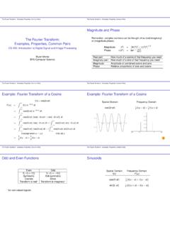
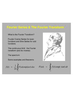
2 Its transform is a Bessel function, (6) to G(u,v)=g(x,y)e i2 (xu+yv)dxdy g(x,y)=G(u,v)ei2 (xu+yv)dudv e (x2+y2)FT e (u2+v2) (x) (y)FT 1 rect(x)rect(y)FT sinc(u)sinc(v) circ(r)FT J1(2 ) The function rect(x)rect(y) is shown on the left. Its transform is the function sinc(u)sinc(v) shown on the right. (Ignore the units in the axes, they are the units of the discrete FT used to make the figure.) 2 here the variables r and represent , respectively. Again, as in the case of the rect function, something with "sharp edges" in one domain transforms into something with ripples in the other. The 2D FT has a set of properties just like the 1D transform.

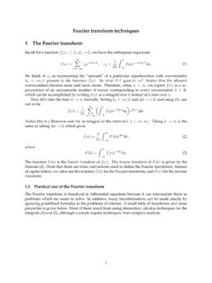
3 1. Linearity 2. Scale 3. Shift 4. Convolution 5. Rotation , where are rotated about the origin through the same angle. The rotation property is the only one we haven t seen before. You can understand it this way: if we define the vectors and then we can rewrite the definition of the FT (eqn. 13) as (7) where the vectors appear only through a dot product in the exponential function. Thus if you rotate the coordinate system for x, a corresponding rotation of u will give the same result for the dot product. (x2+y2)1/2 and (u2+v2)1/2 g+hFT G+H g(ax,by)FT 1abGua,vb g(x a,y b)FT G(u,v)e i2 (au+bv) g hFT G H g( x , y )FT G( u , v ) ( x , y ) and ( u , v )x=(x,y)u=(u,v)G(u)=g(x)e i2 x udx The circ function (shown on the left) has the transform on the right (a Bessel function, also known as the Airy function.)

4 The Airy function is circularly symmetric, but doesn t quite look like that here because of aliasing artifacts from the discrete FFT on a computer (more about that later). 3 More formally, let R be a rotation matrix. Then the FT of a rotated function can be gotten through the substitution in this way: Like the 1D lattice, a 2D lattice with unit spacing transforms into the same function in the other domain. Making use of the scaling rule, it is then easy to show that the general 2D lattice transforms this way: (8) This means that a lattice with spacings 1/a and 1/b transforms to a lattice with spacings a and b, respectively. This is the origin of the term "reciprocal space" for the Fourier transform space.

5 2D Power spectrum The 2D power spectrum is an important tool in electron microscopy. Recall from last time that the power spectrum is the magnitude squared of the FT, so in 2D it is ( , )=| ( , )|*. (9) If the random signal has been filtered by some filter function H such that = , then the expectation value of the spectrum is given by ( , )=| ( , )|*| ( , )|* (10) Let s let H be the contrast transfer function. In two dimensions the CTF should be circularly symmetric (why do you think?) We ll define the magnitude s of the spatial frequency as = *+ * so the CTF has the form ignoring spherical aberration but including the envelope function ( )=sin ( * ) :;<=/?

6 (11) g(Rx)x'=RxGR(u)=g(Rx)e i2 x udx =g( x)e i2 (R 1 x) ud x =g( x)e i2 x (Ru)d x =G(Ru) (ax n)n= (by m)m= FT 1ab ua n n= vb m m= 4 Below left is the theoretical CTF, the middle is a micrograph, and on the right is the power spectrum of the micrograph. Note that the power spectrum looks a lot like the CTF (actually according to (10) it is proportional to the CTF squared). The 2D FT and diffraction The diffraction pattern is the Fourier transform of the amplitude pattern of a source of radiation. Consider the following system. A plane wave is propagating in the +z direction, passing through a scattering object at z=0, where its amplitude becomes Ao(x,y).

7 We want to know the amplitude of the wave at the detector in the u,v plane, which is a distance z from the x,y plane. Classical wave theory says that we can solve this problem by treating each point in the x,y plane as the source of a spherical wavefront. Here is the wave function of a spherical wave of magnitude A0 that starts from the origin, , and the wave function at the detector plane is gotten by adding up a spherical wave emanating from each point in the x,y plane. Using the weak-phase approximation we ll scale the amplitude of each diffracted wave by 1/ and get: D( , )=E G( , ) J( )*+( )*+ * L*MJ(N:O)=P(Q:R)=/S O,R . Making various approximations, specifically assuming u and v are large compared to x and y and that z is much larger than all other dimensions, the Fraunhofer formula for the wave amplitude at the detector plane is (r)=A0rei2 r/ 5 (12) or, letting G be the Fourier transform of the amplitude distribution A(x,y), (13) Where G is the Fourier transform of the amplitude distribution.

8 The intensity of X-rays or photons at the detector will be the squared magnitude of , in which the various phase factors drop out and we have (14) The intensity at the detector is proportional to the magnitude squared of the FT of the scattering pattern. This is the basis of electron crystallography. Working from the measured intensity at the detector, the first step is to find what the amplitude is at the detector (which you get by taking the square root of the intensity and assigning phases). Then the IFT give you the original pattern of amplitudes Ao at the object. The 3D Fourier transform In the same way, there exists a 3D Fourier transform as well. It is defined as a triple integral, and it has all the properties of the 2D FT, including rotations.

9 (15) Central to the theory of 3D reconstruction is the "central slice theorem". It is based on the fact that for any 3D distribution of density g(x,y,z) there is a 3D Fourier transform volume G(u,v,w). If you take a projection through g to obtain a 2D image, it turns out that the Fourier transform of that image has the same values as slice through G. If you have data to fill up the Fourier volume with slices, then you can do an inverse transform to obtain the density map g. We ll talk more about this next time. Discrete Fourier transform and terminology In this course we will be talking about computer processing of images and volumes involving Fourier transforms . The computer operates on data that have been sampled at regular, finite intervals and produces results that we view as individual pixels or voxels.

10 There is an alternative Fourier transform in which the integrals are replaced by sums for working on such finite data sets. This is called the discrete Fourier transform (DFT). Its theory and use are very similar to those of the continuous FT that we have discussed here. There are some considerations about sampling intervals that have to be made, but otherwise things work just fine. In the 1960s people discovered a beautiful algorithm for computing the DFT that is extremely efficient. It is called the fast Fourier transform. Its results are exactly the same as the DFT, only obtained much d(u,v)=ei2 z/ i zei2 (u2+v2)/2 zAo(x,y)e i2 xu+yv()/ zdxdy(x,y) d(u,v)=ei2 z/ i zei (u2+v2)/ z Gu z,v z()A0(x,y) dI(u,v)=1 zGu z,v z 2G(u,v,w)=g(x,y,z)e i2 (xu+yv+wz)dxdy dz 6 more quickly.