Transcription of 3. ANALYTICAL KINEMATICS
1 AME 352 ANALYTICAL KINEMATICS Nikravesh 3-1 3. ANALYTICAL KINEMATICS In planar mechanisms, kinematic analysis can be performed either analytically or graphically. In this course we first discuss ANALYTICAL kinematic analysis. ANALYTICAL KINEMATICS is based on projecting the vector loop equation(s) of a mechanism onto the axes of a non-moving Cartesian frame. This projection transforms a vector equation into two algebraic equations . Then, for a given value of the position (or orientation) of the input link, the algebraic equations are solved for the position/orientation of the remaining links.
2 The first and second time derivative of the algebraic position equations provide the velocity and acceleration equations for the mechanism. For given values of the velocity and acceleration of the input link, these equations are solved to find the velocity and acceleration of the other links in the system. ANALYTICAL KINEMATICS is a systematic process that is most suitable for developing into a computer program. However, for very simple systems, ANALYTICAL kinemtics can be performed by hand calculation. As it will be seen in the upcoming examples, even simple mechanisms can become a challenge for analysis without the use of a computer program.
3 As a reminder, by definition, a mechanism is a collection of links that are interconnected by kinematic joints forming a single degree-of-freedom system. Therefore, in a kinematic analysis, the position, velocity, and acceleration of the input link must be given or assumed (one coordinate, one velocity and one acceleration). The task is then to compute the other coordinates, velocities, and accelerations. Slider-crank (inversion 1) In a slider-crank mechanism, depending on its application, either the crank is the input link and the objective is to determine the KINEMATICS of the connecting rod and the slider, or the slider is the input link and the objective is to determine the KINEMATICS of the connecting rod and the crank.
4 In this example, we assume the first case: For known values of 2, 2, and 2 we want to determine the KINEMATICS of the other links. ABRBAO2 RAO2 RBO2 3 2 We start the analysis by defining vectors and constructing the vector loop equation: RAO2+RBA RBO2=0 The constant lengths are: RAO2=L2, RBA=L3. We place the x-y frame at a convenient location. We define an angle (orientation) for each vector according to our convention (CCW with respect to the positive x-axis). Position equations The vector loop equation is projected onto the x and y axes to obtain two algebraic equations RAO2cos 2+RBAcos 3 RBO2cos 1=0 RAO2sin 2+RBAsin 3 RBO2sin 1=0 Since 1=0, we have: L2cos 2+L3cos 3 RBO2=0L2sin 2+L3sin 3=0 ( ) For known values of L2 and L3, and given value for 2, these equations can be solved 3 and RBO2: sin 3= (L2/L3)sin 2 3=sin 1 3 RBO2=L2cos 2+L3cos 3 AME 352 ANALYTICAL KINEMATICS Nikravesh 3-2 Velocity equations The time derivative of the position equations yields the velocity equations .
5 L2sin 2 2 L3sin 3 3 RBO2=0L2cos 2 2+L3cos 3 3=0 ( ) These equations can also be represented in matrix form, where the terms associated with the known crank velocity are moved to the right-hand-side: L3sin 3 1L3cos 30 3 RBO2 =L2sin 2 2 L2cos 2 2 ( ) Solution of these equations provides values of 3 and RBO2. Acceleration equations The time derivative of the velocity equations yields the acceleration equations : L2sin 2 2 L2cos 2 22 L3sin 3 3 L3cos 3 32 RBO2=0L2cos 2 2 L2sin 2 22+L3cos 3 3 L3sin 3 32=0 ( ) These equations can also be represented in matrix form, where the terms associated with the known crank acceleration and the quadratic velocity terms are moved to the right-hand-side: L3sin 3 1L3cos 30 3 RBO2 =L2(sin 2 2+cos 2 22)+L3cos 3 32 L2(cos 2 2 sin 2 22)+L3sin 3 32 ( ) Solution of these equations provides values of 3 and RBO2.
6 Kinematic analysis For the slider-crank mechanism consider the following constant lengths: L2= and L3= (SI units). For 2=65o, 2= rad/sec, and 2=0, solve the position, velocity and acceleration equations for the unknowns. Position analysis For 2=65o, we need to solve the position equations for 3 and RBO2. Substituting the known values in equations ( ), we have (65)+ 3 RBO2= (65)+ 3=0 (a) The second row of the equation that simplifies to sin 3= (65) 3=sin 1 () 3= ( ) or There are two solutions for 3. Substituting any of these values in the first equation of (a) yields the position of the slider: RBO2= (65)+ ( )= for 3= RBO2= (65)+ ( )= for 3= 335 o 65 o 65 204 o o AME 352 ANALYTICAL KINEMATICS Nikravesh 3-3 The two solutions are shown in the diagram.
7 We select the solution that fits our application here we select the first solution and continue with the rest of the kinematic analysis. Velocity analysis For 2=65o, 3= , RBO2= , and 2= rad/sec, the velocity equations in ( ) become 0 3 RBO2 = solving these two equations in two unknowns yields 3= rad/sec, RBO2= Acceleration analysis Substituting all the known values for the coordinates and velocities in ( ) provides the acceleration equations as 0 3 RBO2 = solving these equations yields 3= rad/sec2, RBO2= Observations The ANALYTICAL process for the KINEMATICS of the slider-crank mechanism reveals the following observations.
8 A mechanism with a single kinematic loop yields one vector-loop equation. A vector loop equation can be represented as two algebraic position equations . Position equations are non- linear in the coordinates (angles and distances). Non- linear equations are difficult and time consuming to solve by hand. Numerical methods, such as Newton-Raphson, are recommended for solving non- linear algebraic equations . The time derivative of position equations yields velocity equations . Velocity equations are linear in the velocities. The time derivative of velocity equations yields acceleration equations .
9 Acceleration equations are linear in the accelerations. The coefficient matrix of the velocities in the velocity equations and the coefficient matrix of the accelerations in the acceleration equations are identical. This characteristic can be used to simplify the solution process of these equations . Four-bar In a four-bar mechanism, generally for a known angle, velocity and acceleration of the input link, we attempt to find the angles, velocities and accelerations of the other two links The vector loop equation for this four-bar is constructed as RAO2+RBA RBO4 RO4O2=0 The length of the links are RO4O2=L1, RAO2=L2, RBA=L3, RBO4=L4 We place the x-y frame at a convenient location as x y ABRBAO2 RAO2 RBO4RO4O2O4 2 3 4 shown.
10 We define an angle (orientation) for each link according to our convention (CCW with respect to the positive x-axis). AME 352 ANALYTICAL KINEMATICS Nikravesh 3-4 Position equations The vector loop equation is projected onto the x- and y-axes to obtain two algebraic equations : RAO2cos 2+RBAcos 3 RBO4cos 4 RO4O2cos 1=0 RAO2sin 2+RBAsin 3 RBO4sin 4 RO4O2sin 1=0 ( ) Since 1=0 and the link lengths are known constants, the equations are simplified to: L2cos 2+L3cos 3 L4cos 4 L1=0L2sin 2+L3sin 3 L4sin 4=0 ( ) Velocity equations The time derivative of the position equations yields.