Transcription of 4.1 Schr odinger Equation in Spherical Coordinates
1 Schro dinger Equation in Spherical Coordinates p2. i~ t = H , where H = 2m + V. ~ 2. p (~/i) implies i~ t = 2m 2 + V .. R. normalization: d3 r | | 2 = 1. If V is independent of t, a complete set of stationary states 3 n(r, t) = n(r)e iEnt/~, where the spatial wavefunction satisfies the time-independent Schro dinger Equation : ~2 2 + V = E . 2m n n n n An arbitrary state can then be written as a sum over these n(r, t). Spherical symmetry If the potential energy and the boundary conditions are spherically symmetric, it is useful to transform H into Spherical Coordinates and seek solutions to Schro dinger's Equation which can be written as the product of a radial portion and an angular portion: (r, , ) = R(r)Y ( , ), or even R(r) ( ) ( ).
2 This type of solution is known as separation of variables'. Figure - Spherical Coordinates . In Spherical Coordinates , the Laplacian takes the form: . 1 f 1 f 2 f = 2 r2 + 2 sin . r r r r sin . ! 1 2f + . r 2 sin2 2. After some manipulation, the equations for the factors become: d2 2 , = m d 2.. d d . sin sin + l(l + 1) sin2 = m2 , and d d . 2. d dR 2mr r2 [V (r) E]R = l(l + 1)R, dr dr ~2. where m2 and l(l + 1) are constants of separation. The solutions to the angular equations with spherically symmetric boundary conditions are: m = (2 ) 1/2eim.
3 And ml P l m (cos ), where m is restricted to the range l, .., l, |m|. m 2. Pl (x) (1 x ) |m|/2 d Pl (x) is the dx associated Legendre function,' and Pl (x) is the lth Legendre polynomial. The product of and occurs so frequently in quantum mechanics that it is known as a Spherical harmonic: " #1/2. (2l + 1) (l |m|)! Ylm( , ) = eim Plm(cos ), 4 (l + |m|)! where = ( 1)m for m 0 and = 1 for m 0, and the Spherical harmonics are orthonormal: Z Z 2 . 0. d sin d [Ylm( , )] [Ylm 0 ( , )] = ll0 mm0 . 0 0. While the angular part of the wavefunction is Ylm( , ) for all spherically symmetric situations, the radial part varies.
4 The Equation for R can be simplified in form by substituting u(r) = rR(r): " #. 2 2. ~ d u 2. ~ l(l + 1). 2. + V + 2. u = Eu, 2m dr 2m r R 2. with normalization dr |u| = 1. This is now referred to as the radial wave Equation , and would be identical to the one-dimensional Schro dinger Equation were it not for the term r 2 added to V , which pushes the particle away from the origin and is therefore often called the centrifugal potential.'. Let's consider some specific examples. Infinite Spherical well (. 0, r < a V (r) =.)
5 , r > a. The wavefunction = 0 for r > a;. for r < a, the differential Equation is " # . d2 u l(l + 1) 2 u, where k 2mE . = k dr 2 r2 ~. The 'stationary' eigenfunctions of this potential are all bound states, confined to the region r < a. The solutions to this Equation are Bessel functions, specifically the Spherical Bessel and Spherical Neumann functions of order l: u(r) = Arjl (kr) + Brnl (kr), l 1 d sin x where jl (x) ( x)l , x dx x l l 1 d cos x and nl (x) ( x) . x dx x The requirement that the wavefunctions be regular' at the origin eliminates the Neumann function from any region including the origin.
6 The Bessel function is similarly eliminated from any region including . Figure - First four Spherical Bessel functions. The remaining constants, k (substituting for E). and A, are satisfied by requiring that the solution vanish at r = a and normalizing, respectively: jl (ka) = 0 ka = nl , where nl is the nth zero of the lth Spherical Bessel function. Adding the angular portion, the complete time-independent wavefunctions are nlm(r, , ) = Anl jl ( nl r/a)Ylm( , ), ~2 2. where Enl = . 2ma2 nl Hydrogen Atom The hydrogen atom consists of an electron orbiting a proton, bound together by the Coulomb force.
7 While the correct dynamics would involve both particles orbiting about a center of mass position, the mass differential is such that it is a very good approximation to treat the proton as fixed at the origin. The Coulomb potential, V 1r , results in a Schro dinger Equation which has both continuum states (E > 0) and bound states (E < 0), both of which are well-studied sets of functions. We shall neglect the former, the confluent hypergeometric functions, for now, and concentrate on the latter. Including constants, the potential is e2 1 , leading to the following V = 4.
8 0r differential Equation for u: " #. 2 2. ~ d u 2. e 1 2. ~ l(l + 1). 2. + + 2. u = Eu. 2m dr 4 0 r 2m r This Equation can be simplified with two . substitutions: since E < 0, both 2mE. ~. and r are non-negative real variables;. furthermore, is dimensionless. With these substitutions, u( ) satisfies: " #. d2 u 0 l(l + 1) me2. 2. = 1 + 2. u; 0 2.. d 2 0~ . Having simplified this Equation more or less as much as possible, let us now look at the asymptotic behavior: As , the constant term in brackets d 2u dominates, or d 2 u, which is satisfied by u = Ae + Be.
9 The second term is irregular as , so B = 0 u Ae as . Similarly, as 0, the term in brackets 2. 2u dominates, leading to d 2 l(l+1). d 2. u, which is satisfied by u = C l+1 + D l . The second term is irregular at 0, so D = 0 u C l+1 as 0. We might hope that we can now solve the differential Equation by assuming a new functional form for u which explicitly includes both kinds of asymptotic behavior: let u( ) l+1e v( ). The resulting differential Equation for v is d2 v dv 2 + 2(l + 1 ) + [ 0 2(l + 1)]v = 0. d d . Furthermore, let us assume that v( ) can be expressed as a power series in.
10 X. v( ) = aj j . j=0. The problem then becomes one of solving for {aj }. If we had expanded in a series of orthonormal functions, it would now be possible to substitute that series into the differential Equation and set the coefficients of each term equal to zero. Powers of are not orthonormal, however, so we must use a more difficult argument based on the Equation holding for all values of to group separately the coefficients for each power of : " #. 2(j + l + 1) 0. aj+1 = aj . (j + 1)(j + 2l + 2). Let's examine the implications of this recursion relation for the solutions to the Schro dinger Equation .