4.15 Three Factor Factorial Designs complete interaction model

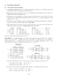
1 Factor Factorial Designs Thecomplete interaction modelfor a Three - Factor completely randomized design is:yijkl=(35) is the baseline mean, i, j, and kare the main Factor effects forA,B, andC, respectively. ( )ij, ( )ikand ( )jkare the two- Factor interaction effects for interactionsAB,AC, andBC, respectively. ( )ijkare the Three - Factor interaction effects for theABCinteraction. eijklis the random error of thekthobservation from the (i,j,k) assumeeijkl IID N(0, 2). For now, we will also assume all effects are Partitioning the total sum of squares SST= ai=1 bj=1 ck=1 nl=1(yijkl y )2 Note that we can rewriteyijklasyijkl= + i+ j+ k+ ( )ij+ ( )ik+ ( )jk+ ( )ijk+eijklwhere =y i=yi y j=y j y k=y k y ( )ij=yij yi y j +y ( )ik=yi k yi y k +y ( )jk=y jk y j y k +y ( )ijk=yijk yij yi k y jk +yi +y j +y k y eijkl=yijkl yijk Substitution of these estimates intoSSTyieldsSST=a i=1b j=1c k=1n l=1(yijkl y )

2 2=a i=1b j=1c k=1n l=1( i+ j+ k+ ( )ij+ ( )ik+ ( )jk+ ( )ijk+eijkl)2=a i=1b j=1c k=1n l=1 2i+a i=1b j=1c k=1n l=1 2j+a i=1b j=1c k=1n l=1 k+a i=1b j=1c k=1n l=1( )2ij+a i=1b j=1c k=1n l=1( )2ik+a i=1b j=1c k=1n l=1( )2jk+a i=1b j=1c k=1n l=1( )2ijk+a i=1b j=1c k=1n l=1e2ijkl+a i=1b j=1c k=1n l=1(all cross-products of parameter estimates)Through tedious algebra, it can be shown cross-products of parameter estimates = of the multiple summations produces:SST=bcna i=1 2i+acnb j=1 2j+abnc k=1 k+cna i=1b j=1( )2ij+bna i=1c k=1( )2ik+anb j=1c k=1( )2jk+na i=1b j=1c k=1( )2ijk+a i=1b j=1c k=1n l=1e2ijkl=SSA+SSB+SSC+SSAB+SSAC+SSBC+SSA BC+SSE161174Ii= iJj= jKk= k(IJ)ij= ij(IK)ik= ik(JK)jk= jk(IJK)ijk= ijkEijkl=eijkl162 Three - Factor Factorial Designs : Fixed factors A, B, C175 Three Factor Factorial Example In a paper production process, the effects of percentage of hardwood concentration in raw wood pulp,the vat pressure, and the cooking time on the paper strength were studied.

3 There werea= 3 levels of hardwood concentration (CONC = 2%, 4%, 8%).There wereb= 3 levels of vat pressure (PRESS = 400, 500, 650).There werec= 2 levels of cooking time (TIME = 3 hours, 4 hours).163 A Three Factor Factorial experiment withn= 2 replicates was run. The order of data collection wascompletely randomized. We assume all Three factors are fixed. The experimental data are in the table time hoursCooking time From the SAS output, thep-value = .2903 is not significant for the test of the equality of the threefactor interaction effects: H0: ijk= 0 for alli,j,kvs H1: ijk6= 0 for somei,j,k Thep-values of.

4 0843, .0146, and .0750 for the CONC*TIME, CONC*PRESS, and TIME*PRESS twofactor interactions are all significant at the =.10 level indicating the interpretation of the significantmain effects for CONC (p-value=.0009), TIME (p-value< .0001), and PRESS (p-value< .0001) maybe masked. To understand the effects in the model , we need to examine the interaction Factor ANALYSIS OF VARIANCEThe GLM ProcedureDependent Variable: strengthTHREE Factor ANALYSIS OF VARIANCEThe GLM ProcedureDependent Variable: strengthSourceDFSum ofSquaresMean SquareF ValuePr> <. VarRoot III SSMean SquareF ValuePr> <.

5 0001conc* <.0001conc* * *time* Factor ANALYSIS OF VARIANCEThe GLM ProcedureTHREE Factor ANALYSIS OF VARIANCEThe GLM Procedure196197198199200201strength40050 0650pressDistribution of strengthstrengthLevelofpressNMeanStd Factor ANALYSIS OF VARIANCEThe GLM Procedure196197198199200201strength248co ncDistribution of strengthstrengthLevelofconcNMeanStd Factor ANALYSIS OF VARIANCEThe GLM ProcedureTHREE Factor ANALYSIS OF VARIANCEThe GLM Procedure196197198199200201strength40050 0650pressDistribution of strengthstrengthLevelofpressNMeanStd Factor ANALYSIS OF VARIANCEThe GLM

6 Procedure196197198199200201strength248co ncDistribution of strengthstrengthLevelofconcNMeanStd Factor ANALYSIS OF VARIANCEThe GLM Procedure196197198199200201strength2 4002 5002 6504 4004 5004 6508 4008 5008 650conc*pressDistribution of strengthstrengthLevelofconcLevelofpressN MeanStd Factor ANALYSIS OF VARIANCEThe GLM Procedure196197198199200201strength34tim eDistribution of strengthstrengthLeveloftimeNMeanStd Factor ANALYSIS OF VARIANCEThe GLM Procedure196197198199200201strength2 4002 5002 6504 4004 5004 6508 4008 5008 650conc*pressDistribution of strengthstrengthLevelofconcLevelofpressN MeanStd Factor ANALYSIS OF VARIANCEThe GLM Procedure196197198199200201strength34tim eDistribution of strengthstrengthLeveloftimeNMeanStd Factor ANALYSIS OF VARIANCEThe GLM Procedure196197198199200201strength3 4003 5003 6504 4004 5004 650time*pressDistribution of strengthstrengthLeveloftimeLevelofpressN MeanStd Factor ANALYSIS OF VARIANCEThe GLM Procedure196197198199200201strength2 32 44 34 48 38 4conc*timeDistribution of strengthstrengthLevelofconcLeveloftimeNM eanStd Factor ANALYSIS OF VARIANCEThe GLM

7 Procedure196197198199200201strength3 4003 5003 6504 4004 5004 650time*pressDistribution of strengthstrengthLeveloftimeLevelofpressN MeanStd Factor ANALYSIS OF VARIANCEThe GLM Procedure196197198199200201strength2 32 44 34 48 38 4conc*timeDistribution of strengthstrengthLevelofconcLeveloftimeNM eanStd Factor ANALYSIS OF VARIANCEThe GLM Procedure196197198199200201strength2 3 4002 3 5002 3 6502 4 4002 4 5002 4 6504 3 4004 3 5004 3 6504 4 4004 4 5004 4 6508 3 4008 3 5008 3 6508 4 4008 4 5008 4 650conc*time*pressDistribution of strengthstrengthLevelofconcLeveloftimeLe velofpressNMeanStd of Normality AssumptionThe UNIVARIATE ProcedureVariable: residCheck of Normality AssumptionThe UNIVARIATE ProcedureVariable: residMomentsN36 Sum Weights36 Mean0 Sum Observations0 Std Error Statistical : The mode displayed is the smallest of 2 modes with a count of :Mu0=0 TestStatisticp ValueStudent's tt0Pr > |t| >= |M| >= |S| for NormalityTestStatisticp < > D< > W-Sq< > of Normality AssumptionThe UNIVARIATE ProcedureVariable.

8 ResidCheck of Normality AssumptionThe UNIVARIATE ProcedureVariable: residMomentsN36 Sum Weights36 Mean0 Sum Observations0 Std Error Statistical : The mode displayed is the smallest of 2 modes with a count of :Mu0=0 TestStatisticp ValueStudent's tt0Pr > |t| >= |M| >= |S| for NormalityTestStatisticp < > D< > W-Sq< > Factor ANALYSIS OF VARIANCEThe GLM ProcedureFit Diagnostics for DF18 Parameters36 ObservationsProportion 's D196197198199200201 Predicted Value-2-1012 RStudent196197198199200201 Predicted Code for Three - Factor Factorial Example**;** Three Factor ANALYSIS OF VARIANCE **;**;DATA in;DO conc = 2 , 4 , 8;DO time = 3 TO 4;DO press= 400 , 500 , 650;DO rep = 1 TO 2;INPUT strength @@;strength=strength + 190; OUTPUT;END; END; END; END;CARDS.

9 GLM DATA=in PLOTS=(ALL);CLASS conc time press; model strength = conc|time|press / SS3;* MEANS press|conc|time@2;MEANS press|conc|time;OUTPUT OUT=diag R=resid;TITLE Three Factor ANALYSIS OF VARIANCE ;PROC UNIVARIATE DATA=diag NORMAL PLOTS;VAR resid;TITLE "Check of Normality Assumption";RUN; Factor Factorial ANOVA with BlocksEXAMPLE: The yield of a chemical process is being studied. The two factors of interest are Temperature and Pressure. Three levels of each Factor (a= 3,b= 3)are selected.

10 Only nine runs can be made in one day. The experimenter runs a complete replicate of the two factorfactorial design on each day. The data are shown in the following table. Analyze the data assuming that the days are blocks. You just have to add a block effect (DAY) to the two Factor Factorial 1 Day Factorial WITH BLOCKSThe GLM ProcedureDependent Variable: yieldTWO- Factor Factorial WITH BLOCKSThe GLM ProcedureDependent Variable: yieldSourceDFSum ofSquaresMean SquareF ValuePr> <. VarRoot III SSMean SquareF ValuePr> <. * Factorial WITH BLOCKSThe GLM ProcedureTWO- Factor Factorial WITH BLOCKSThe GLM ProcedureSourceType III Expected Mean SquaretempVar(Error) + Q(temp,temp*press)pressVar(Error) + Q(press,temp*press)temp*pressVar(Error) + Q(temp*press)dayVar(Error) + 9 Var(day)TWO- Factor Factorial WITH BLOCKSThe GLM ProcedureTests of Hypotheses for Mixed model Analysis of VarianceDependent Variable: yieldTWO- Factor Factorial WITH BLOCKSThe GLM ProcedureTests of Hypotheses for Mixed model Analysis of VarianceDependent Variable: yi