Transcription of 5: Introduction to Estimation - San Jose State University
1 Page (C:\Users\B. Burt Gerstman\Dropbox\StatPrimer\ , 5/8/2016) 5: Introduction to Estimation Contents Acronyms and symbols .. 1 Statistical inference .. 2 Estimating with confidence .. 3 Sampling distribution of the mean .. 3 Confidence Interval for when is known before hand .. 4 Sample Size Requirements for estimating with confidence .. 6 Estimating p with 7 Sampling distribution of the proportion .. 7 Confidence interval for p .. 7 Sample size requirement for estimating p with confidence .. 9 Acronyms and symbols q complement of the sample proportion x sample mean p sample proportion 1 confidence level CI confidence interval LCL lower confidence limit m margin of error n sample size NHTS null hypothesis test of significance p binomial success parameter ( population proportion ) s sample standard deviation SDM sampling distribution of mean (hypothetical probability model) SEM standard error of the mean SEP standard error of the proportion UCL upper confidence limit alpha level expected value ( population mean ) standard deviation parameter Page (C:\Users\B.)
2 Burt Gerstman\Dropbox\StatPrimer\ , 5/8/2016) Statistical inference Statistical inference is the act of generalizing from the data ( sample ) to a larger phenomenon ( population ) with calculated degree of certainty. The act of generalizing and deriving statistical judgments is the process of inference. [Note: There is a distinction between causal inference and statistical inference. Here we consider only statistical inference.] The two common forms of statistical inference are: Estimation Null hypothesis tests of significance (NHTS) There are two forms of Estimation : Point Estimation (maximally likely value for parameter) Interval Estimation (also called confidence interval for parameter) This chapter introduces Estimation . The following chapter introduced NHTS. Both Estimation and NHTS are used to infer parameters.
3 A parameter is a statistical constant that describes a feature about a phenomena, population, pmf, or pdf. Examples of parameters include: Binomial probability of success p (also called the population proportion ) Expected value (also called the population mean ) Standard deviation (also called the population standard deviation ) Point estimates are single points that are used to infer parameters directly. For example, Sample proportionp ( p hat ) is the point estimator of p Sample mean x ( x bar ) is the point estimator of Sample standard deviation s is the point estimator of Notice the use of different symbols to distinguish estimators and parameters. More importantly, point estimates and parameters represent fundamentally different things. Point estimates are calculated from the data; parameters are not.
4 Point estimates vary from study to study; parameters do not. Point estimates are random variables: parameters are constants. Page (C:\Users\B. Burt Gerstman\Dropbox\StatPrimer\ , 5/8/2016) Estimating with confidence Sampling distribution of the mean Although point estimate x is a valuable reflections of parameter , it provides no information about the precision of the estimate. We ask: How precise is x as estimate of ? How much can we expect any given x to vary from ? The variability of x as the point estimate of starts by considering a hypothetical distribution called the sampling distribution of a mean (SDM for short). Understanding the SDM is difficult because it is based on a thought experiment that doesn t occur in actuality, being a hypothetical distribution based on mathematical laws and probabilities.
5 The SDM imagines what would happen if we took repeated samples of the same size from the same (or similar) populations done under the identical conditions. From this hypothetical experiment we build a pmf or pdf that is used to determine probabilities for various hypothetical outcomes. Without going into too much detail, the SDM reveals that: x is an unbiased estimate of ; the SDM tends to be normal (Gaussian) when the population is normal or when the sample is adequately large; the standard deviation of the SDM is equal to n . This statistic which is called the standard error of the mean (SEM) predicts how closely the sx in the SDM are likely to cluster around the value of and is a reflection of the precision of x as an estimate of : nSEM = Note that this formula is based on and not on sample standard deviation s.
6 Recall that is NOT calculated from the data and is derived from an external source. Also note that the SEM is inversely proportion to the square root of n. Numerical example. Suppose a measurement that has = 10. o A sample of n = 1 for this variable derives SEM = n = 10 / 1 = 10 o A sample of n = 4 derives SEM = n = 10 / 4 = 5 o A sample of n = 16 derives SEM = n = 10 / 16 = Each time we quadruple n, the SEM is cut in half. This is called the square root law the precision of the mean is inversely proportional to the square root of the sample size. Page (C:\Users\B. Burt Gerstman\Dropbox\StatPrimer\ , 5/8/2016) Confidence Interval for when is known before hand To gain further insight into , we surround the point estimate with a margin of error: This forms a confidence interval (CI).
7 The lower end of the confidence interval is the lower confidence limit (LCL). The upper end is the upper confidence limit (UCL). Note: The margin of error is the plus-or-minus wiggle-room drawn around the point estimate; it is equal to half the confidence interval length. Let (1 )100% represent the confidence level of a confidence interval. The ( alpha ) level represents the lack of confidence and is the chance the researcher is willing to take in not capturing the value of the parameter. A (1 )100% CI for is given by: ))((2/1 SEMzx The z1- /2 in this formula is the z quantile association with a 1 level of confidence. The reason we use z1- /2 instead of z1- in this formula is because the random error (imprecision) is split between underestimates (left tail of the SDM) and overestimates (right tail of the SDM).
8 The confidence level 1 area lies between z1 /2 and z1 /2: Page (C:\Users\B. Burt Gerstman\Dropbox\StatPrimer\ , 5/8/2016) You may use the z/t table on the StatPrimer website to determine z quantiles for various levels of confidence. Here are the common levels of confidence and their associated alpha levels and z quantiles: (1 )100% z1- /2 90% .10 95% .05 99% .01 Numerical example, 90% CI for . Suppose we have a sample of n = 10 with SEM = andx = The z quantile for 10% confidence is z1 .10/2 = = and the 90% CI for = ( )( ) = = ( , ). We use this inference to address population mean and NOT about sample mean x. Note that the margin of error for this estimate is Numerical example, 95% CI for . The z quantile for 95% confidence is z1 .05/2 = = The 95% CI for = ( )( ) = = ( , ).
9 Note that the margin of error for this estimate is Numerical example, 99% CI for . Using the same data, = .01 for 99% confidence and the 99% CI for = ( )( ) = = ( , ). Note that the margin of error for this estimate is Here are confidence interval lengths (UCL LCL) of the three intervals just calculated: Confidence Level Confidence Interval Confidence Interval Length 90% ( , ) = 95% ( , ) = 99% ( , ) = The confidence interval length grows as the level of confidence increases from 90% to 95% to 99%.This is because there is a trade-off between the confidence and margin of error. You can achieve a smaller margin of error if you are willing to pay the price of less confidence. Therefore, as Dr. Evil might say, 95% is pretty standard.
10 Numerical example. Suppose a population has = 15 (not calculated, but known ahead of time) and unknown mean . We take a random sample of 10 observations from this population and observe the following values: {21, 42, 5, 11, 30, 50, 28, 27, 24, 52}. Based on these 10 observations, x= , SEM = 15/ 10 = and a 95% CI for = ( )( ) = = ( , ). Interpretation notes: The margin of error (m) is the plus or minus value surrounding the estimate. In this case m = We use these confidence interval to address potential locations of the population mean , NOT the sample mean x. Page (C:\Users\B. Burt Gerstman\Dropbox\StatPrimer\ , 5/8/2016) Sample Size Requirements for estimating with confidence One of the questions we often faces is How much data should be collected?