Transcription of 7.1 Vectors, Tensors and the Index Notation - Auckland
1 Section Vectors, Tensors and the Index Notation The equations governing three dimensional mechanics problems can be quite lengthy. For this reason, it is essential to use a short-hand Notation called the Index Notation 1. Consider first the Notation used for vectors. Vectors Vectors are used to describe physical quantities which have both a magnitude and a direction associated with them. Geometrically, a vector is represented by an arrow; the arrow defines the direction of the vector and the magnitude of the vector is represented by the length of the arrow. Analytically, in what follows, vectors will be represented by lowercase bold-face Latin letters, a, b. The dot product of two vectors a and b is denoted by a b and is a scalar defined by a b = a b cos . ( ). here is the angle between the vectors when their initial points coincide and is restricted to the range 0 . Cartesian Coordinate System So far the short discussion has been in symbolic Notation 2, that is, no reference to axes'.
2 Or components' or coordinates' is made, implied or required. Vectors exist independently of any coordinate system. The symbolic Notation is very useful, but there are many circumstances in which use of the component forms of vectors is more helpful . or essential. To this end, introduce the vectors e1 , e 2 , e 3 having the properties e1 e 2 = e 2 e 3 = e 3 e1 = 0 , ( ). so that they are mutually perpendicular, and e1 e1 = e 2 e 2 = e 3 e 3 = 1 , ( ). so that they are unit vectors. Such a set of orthogonal unit vectors is called an orthonormal set, Fig. This set of vectors forms a basis, by which is meant that any other vector can be written as a linear combination of these vectors, in the form a = a1e1 + a 2 e 2 + a3 e 3 ( ). where a1 , a 2 and a3 are scalars, called the Cartesian components or coordinates of a along the given three directions. The unit vectors are called base vectors when used for 1.
3 Or indicial or subscript or suffix Notation 2. or absolute or invariant or direct or vector Notation Solid Mechanics Part II 191 Kelly Section this purpose. The components a1 , a 2 and a3 are measured along lines called the x1 , x 2. and x3 axes, drawn through the base vectors. a e3. a3. e2. e1. a1. a2. Figure : an orthonormal set of base vectors and Cartesian coordinates Note further that this orthonormal system {e1 , e 2 , e 3 } is right-handed, by which is meant e1 e 2 = e 3 (or e 2 e 3 = e1 or e 3 e1 = e 2 ). In the Index Notation , the expression for the vector a in terms of the components a1 , a 2 , a3. and the corresponding basis vectors e1 , e 2 , e 3 is written as 3. a = a1e1 + a 2 e 2 + a3 e 3 = ai e i ( ). i =1. This can be simplified further by using Einstein's summation convention, whereby the summation sign is dropped and it is understood that for a repeated Index (i in this case) a summation over the range of the Index (3 in this case 3) is implied.
4 Thus one writes a = ai e i . This can be further shortened to, simply, ai . The dot product of two vectors u and v, referred to this coordinate system, is u v = (u1e1 + u 2 e 2 + u 3 e 3 ) (v1e1 + v 2 e 2 + v3 e 3 ). = u1v1 (e1 e1 ) + u1v 2 (e1 e 2 ) + u1v3 (e1 e 3 ). + u 2 v1 (e 2 e1 ) + u 2 v 2 (e 2 e 2 ) + u 2 v3 (e 2 e 3 ) ( ). + u 3 v1 (e 3 e1 ) + u 3 v 2 (e 3 e 2 ) + u 3 v3 (e 3 e 3 ). = u1v1 + u 2 v 2 + u 3 v3. The dot product of two vectors written in the Index Notation reads u v = u i vi Dot Product ( ). 3. 2 in the case of a two-dimensional space/analysis Solid Mechanics Part II 192 Kelly Section The repeated Index i is called a dummy Index , because it can be replaced with any other letter and the sum is the same; for example, this could equally well be written as u v = u j v j or u k v k . Introduce next the Kronecker delta symbol ij , defined by 0, i j ij = ( ). 1, i = j Note that 11 = 1 but, using the Index Notation , ii = 3.
5 The Kronecker delta allows one to write the expressions defining the orthonormal basis vectors ( , ) in the compact form e i e j = ij Orthonormal Basis Rule ( ). Example Recall the equations of motion, Eqns. , which in full read 11 12 13. + + + b1 = a1. x1 x 2 x3. 21 22 23. + + + b2 = a 2 ( ). x1 x 2 x3. 31 32 33. + + + b3 = a3. x1 x 2 x3. The Index Notation for these equations is ij + bi = ai ( ). x j Note the dummy Index j. The Index i is called a free Index ; if one term has a free Index i, then, to be consistent, all terms must have it. One free Index , as here, indicates three separate equations. Matrix Notation The symbolic Notation v and Index Notation vi e i (or simply vi ) can be used to denote a vector . Another Notation is the matrix Notation : the vector v can be represented by a 3 1 matrix (a column vector ): Solid Mechanics Part II 193 Kelly Section v1 . v . 2 . v3 . Matrices will be denoted by square brackets, so a shorthand Notation for this matrix/ vector would be [v ].
6 The elements of the matrix [v ] can be written in the Index Notation vi . Note the distinction between a vector and a 3 1 matrix: the former is a mathematical object independent of any coordinate system, the latter is a representation of the vector in a particular coordinate system matrix Notation , as with the Index Notation , relies on a particular coordinate system. As an example, the dot product can be written in the matrix Notation as v1 . [u ][v] = [u T. 1 u2 u 3 ] v 2 . v3 . short . matrix Notation full . matrix Notation [ ]. Here, the Notation u T denotes the 1 3 matrix (the row vector ). The result is a 1 1. matrix, u i vi . The matrix Notation for the Kronecker delta ij is the identity matrix 1 0 0 . [I ] = 0 1 0 . 0 0 1 . Then, for example, in both Index and matrix Notation : 1 0 0 u1 u1 . ij u j = u i [I ][u] = [u] 0 1 0 u = u ( ). 2 2 . 0 0 1 u 3 u 3 . Matrix Matrix Multiplication When discussing vector transformation equations further below, it will be necessary to multiply various matrices with each other (of sizes 3 1 , 1 3 and 3 3 ).
7 It will be helpful to write these matrix multiplications in the short-hand Notation . Solid Mechanics Part II 194 Kelly Section [ ]. First, it has been seen that the dot product of two vectors can be represented by u T [v ] or [ ]. u i vi . Similarly, the matrix multiplication [u ] v T gives a 3 3 matrix with element form u i v j or, in full, u1v1 u1v 2 u1v3 . u v 2 1 u 2 v2 u 2 v3 . u 3 v1 u3v2 u 3 v3 . This operation is called the tensor product of two vectors, written in symbolic Notation as u v (or simply uv). Next, the matrix multiplication Q11 Q12 Q13 u1 . [Q][u] Q21 Q22 Q23 u 2 . Q31 Q32 Q33 u 3 . is a 3 1 matrix with elements ([Q][u ])i Qij u j . The elements of [Q][u] are the same as [ ][ ]. those of u T Q T , which can be expressed as ( u T Q T [ ][ ]) i u j Qij . [ ]. The expression [u][Q] is meaningless, but u T [Q] { Problem 4} is a 1 3 matrix with [ ]. elements ( u T [Q])i u j Q ji.
8 This leads to the following rule: 1. if a vector pre-multiplies a matrix [Q] the vector is the transpose u T [ ]. 2. if a matrix [Q] pre-multiplies the vector the vector is [u ]. 3. if summed indices are beside each other , as the j in u j Q ji or Qij u j the matrix is [Q]. 4. if summed indices are not beside each other, as the j in u j Qij the matrix is the transpose, Q T [ ]. Finally, consider the multiplication of 3 3 matrices. Again, this follows the beside each other rule for the summed Index . For example, [A ][B ] gives the 3 3 matrix [ ]. { Problem 8} ([A ][B ])ij = Aik Bkj , and the multiplication A T [B ] is written as ([A ][B]). T. ij = Aki Bkj . There is also the important identity ([A][B])T [ ][ ]. = BT AT ( ). Note also the following: Solid Mechanics Part II 195 Kelly Section (i) if there is no free Index , as in u i vi , there is one element (ii) if there is one free Index , as in u j Q ji , it is a 3 1 (or 1 3 ) matrix (iii) if there are two free indices, as in Aki Bkj , it is a 3 3 matrix vector Transformation Rule Introduce two Cartesian coordinate systems with base vectors e i and e i and common origin o, Fig.
9 The vector u can then be expressed in two ways: u = u i e i = u i e i ( ). x2. x2 . u1 . u2 . u x1 u2.. e 2 e1 .. o x1. u1. Figure : a vector represented using two different coordinate systems Note that the xi coordinate system is obtained from the xi system by a rotation of the base vectors. Fig. shows a rotation about the x3 axis (the sign convention for rotations is positive counterclockwise). Concentrating for the moment on the two dimensions x1 x 2 , from trigonometry (refer to Fig. ), u = u1e1 + u 2 e 2. = [ OB AB ]e1 + [ BD + CP ]e 2 ( ). = [cos u1 sin u 2 ]e1 + [sin u1 + cos u 2 ]e 2. and so u1 = cos u1 sin u2 . ( ). u2 = sin u1 + cos u2 . vector components in vector components in first coordinate system second coordinate system Solid Mechanics Part II 196 Kelly Section x2. x2 . u1 P. u2 .. x1 u2. C. D. A B. x1. o u1. Figure : geometry of the 2D coordinate transformation In matrix form, these transformation equations can be written as u1 cos sin u1.
10 U = sin ( ). 2 cos u 2 . The 2 2 matrix is called the transformation matrix or rotation matrix [Q] . By pre- multiplying both sides of these equations by the inverse of [Q] , Q 1 , one obtains the [ ]. transformation equations transforming from [u1 u 2 ] to [u1 u 2 ] : T T. u1 cos sin u1 . u = sin ( ). 2 cos u 2 . It can be seen that the components of [Q] are the directions cosines, the cosines of the angles between the coordinate directions: Qij = cos(xi , x j ) = e i e j ( ). It is straight forward to show that, in the full three dimensions, Fig. , the components in the two coordinate systems are also related through u i = Qij u j [u] = [Q][u ]. vector Transformation Rule ( ). u i = Q ji u j [u ] = [Q T ][u]. Solid Mechanics Part II 197 Kelly Section x2. x2 . u x1 . x1. x3 . x3. Figure : two different coordinate systems in a 3D space Orthogonality of the Transformation Matrix [Q].