Transcription of 7 The Backpropagation Algorithm - fu-berlin.de
1 R. Rojas: Neural Networks, Springer-Verlag, Berlin, 19967 The Backpropagation Learning as gradient descentWe saw in the last chapter that multilayered networks are capable of com-puting a wider range of Boolean functions than networks witha single layerof computing units. However the computational effort neededfor finding thecorrect combination of weights increases substantially when more parametersand more complicated topologies are considered. In this chapter we discuss apopular learning method capable of handling such large learning problems the Backpropagation Algorithm . This numerical method was used by differentresearch communities in different contexts, was discoveredand rediscovered,until in 1985 it found its way into connectionist AI mainly through the work ofthe PDP group [382]. It has been one of the most studied and used algorithmsfor neural networks learning ever this chapter we present a proof of the Backpropagation Algorithm basedon a graphical approach in which the Algorithm reduces to a graph labelingproblem.
2 This method is not only more general than the usual analyticalderivations, which handle only the case of special network topologies, butalso much easier to follow. It also shows how the Algorithm can be efficientlyimplemented in computing systems in which only local information can betransported through the Differentiable activation functionsThe Backpropagation Algorithm looks for the minimum of the error functionin weight space using the method of gradient descent. The combination ofweights which minimizes the error function is considered tobe a solution ofthe learning problem. Since this method requires computation of the gradientof the error function at each iteration step, we must guarantee the conti-nuity and differentiability of the error function. Obviously we have to use akind of activation function other than the step function used in perceptrons,R.
3 Rojas: Neural Networks, Springer-Verlag, Berlin, 1996R. Rojas: Neural Networks, Springer-Verlag, Berlin, 1996R. Rojas: Neural Networks, Springer-Verlag, Berlin, 1996152 7 The Backpropagation Algorithmbecause the composite function produced by interconnectedperceptrons isdiscontinuous, and therefore the error function too. One ofthe more popu-lar activation functions for Backpropagation networks is thesigmoid, a realfunctionsc: IR (0,1) defined by the expressionsc(x) =11 + e constantccan be selected arbitrarily and its reciprocal 1/cis calledthe temperature parameter in stochastic neural networks. The shape of thesigmoid changes according to the value ofc, as can be seen in Figure Thegraph shows the shape of the sigmoid forc= 1,c= 2 andc= 3. Highervalues ofcbring the shape of the sigmoid closer to that of the step functionand in the limitc the sigmoid converges to a step function at the order to simplify all expressions derived in this chapterwe setc= 1, butafter going through this material the reader should be able to generalize allthe expressions for a variablec.
4 In the following we call the sigmoids1(x) justs(x).-4-2024x1 Fig. sigmoids (forc= 1,c= 2 andc= 3)The derivative of the sigmoid with respect tox, needed later on in thischapter, isddxs(x) =e x(1 + e x)2=s(x)(1 s(x)).We have already shown that, in the case of perceptrons, a symmetrical activa-tion function has some advantages for learning. An alternative to the sigmoidis the symmetrical sigmoidS(x) defined asS(x) = 2s(x) 1 =1 e x1 + e is nothing but the hyperbolic tangent for the argumentx/2 whose shapeis shown in Figure (upper right). The figure shows four types of continuous squashing functions. The ramp function (lower right) can also be used inR. Rojas: Neural Networks, Springer-Verlag, Berlin, 1996R. Rojas: Neural Networks, Springer-Verlag, Berlin, 1996R. Rojas: Neural Networks, Springer-Verlag, Berlin, Learning as gradient descent 153learning algorithms taking care to avoid the two points where the derivativeis of some squashing functionsMany other kinds of activation functions have been proposedand the back-propagation Algorithm is applicable to all of them.
5 A differentiable activationfunction makes the function computed by a neural network differentiable (as-suming that the integration function at each node is just thesum of theinputs), since the network itself computes only function compositions. Theerror function also becomes shows the smoothing produced by a sigmoid in a stepof the errorfunction. Since we want to follow the gradient direction to find the minimum ofthis function, it is important that no regions exist in whichthe error functionis completely flat. As the sigmoid always has a positive derivative, the slope ofthe error function provides a greater or lesser descent direction which can befollowed. We can think of our search Algorithm as a physical process in whicha small sphere is allowed to roll on the surface of the error function until itreaches the Regions in input spaceThe sigmoid s output range contains all numbers strictly between 0 and extreme values can only be reached asymptotically.
6 Thecomputing unitsconsidered in this chapter evaluate the sigmoid using the net amount of exci-tation as its argument. Given weightsw1,..,wnand a bias , a sigmoidalunit computes for the inputx1,..,xnthe output11 + exp ( ni=1wixi ).R. Rojas: Neural Networks, Springer-Verlag, Berlin, 1996R. Rojas: Neural Networks, Springer-Verlag, Berlin, 1996R. Rojas: Neural Networks, Springer-Verlag, Berlin, 1996154 7 The Backpropagation AlgorithmFig. step of the error functionA higher net amount of excitation brings the unit s output nearer to 1. Thecontinuum of output values can be compared to a division of the input spacein a continuum of classes. A higher value ofcmakes the separation in inputspace sharper.(0,0)(0,1)(1,0)(1,1)weightFig. of classes in input spaceNote that the step of the sigmoid is normal to the vector (w1.)
7 ,wn, )so that the weight vector points in the direction in extendedinput space inwhich the output of the sigmoid changes Local minima of the error functionA price has to be paid for all the positive features of the sigmoid as activationfunction. The most important problem is that, under some circumstances,local minima appear in the error function which would not be there if thestep function had been used. Figure shows an example of a local minimumwith a higher error level than in other regions. The functionwas computedfor a single unit with two weights, constant threshold, and four input-outputpatterns in the training set. There is a valley in the error function and ifR. Rojas: Neural Networks, Springer-Verlag, Berlin, 1996R. Rojas: Neural Networks, Springer-Verlag, Berlin, 1996R. Rojas: Neural Networks, Springer-Verlag, Berlin, General feed-forward networks 155gradient descent is started there the Algorithm will not converge to the local minimum of the error functionIn many cases local minima appear because the targets for theoutputsof the computing units are values other than 0 or 1.
8 If a network for thecomputation of XOR is trained to produce at the inputs (0,1) and (1,0)then the surface of the error function develops some protuberances, wherelocal minima can arise. In the case of binary target values some local minimaare also present, as shown by Lisboa and Perantonis who analytically foundall local minima of the XOR function [277]. General feed-forward networksIn this section we show that Backpropagation can easily be derived by linkingthe calculation of the gradient to a graph labeling approach isnot only elegant, but also more general than the traditionalderivations foundin most textbooks. General network topologies are handled right from thebeginning, so that the proof of the Algorithm is not reduced to the multilayeredcase. Thus one can have it both ways, more general yet simpler[375].
9 The learning problemRecall that in our general definition a feed-forward neural network is a com-putational graph whose nodes are computing units and whose directed edgestransmit numerical information from node to node. Each computing unit is ca-pable of evaluating a single primitive function of its input. In fact the networkrepresents a chain of function compositions which transform an input to anoutput vector (called a pattern). The network is a particular implementationof a composite function from input to output space, which we call thenetworkfunction. The learning problem consists of finding the optimal combinationR. Rojas: Neural Networks, Springer-Verlag, Berlin, 1996R. Rojas: Neural Networks, Springer-Verlag, Berlin, 1996R. Rojas: Neural Networks, Springer-Verlag, Berlin, 1996156 7 The Backpropagation Algorithmof weights so that the network function approximates a given functionfas closely as possible.
10 However, we are not given the functionfexplicitlybutonly implicitly through some a feed-forward network withninput andmoutput units. It canconsist of any number of hidden units and can exhibit any desired feed-forwardconnection pattern. We are also given a training set{(x1,t1),..,(xp,tp)}consisting ofpordered pairs ofn- andm-dimensional vectors, which are calledthe input and output patterns. Let the primitive functions at each node of thenetwork be continuous and differentiable. The weights of theedges are realnumbers selected at random. When the input patternxifrom the training setis presented to this network, it produces an outputoidifferent in general fromthe targetti. What we want is to makeoiandtiidentical fori= 1,..,p,by using a learning Algorithm . More precisely, we want to minimize the errorfunction of the network, defined asE=12p i=1 oi ti minimizing this function for the training set, new unknown input pat-terns are presented to the network and we expect it tointerpolate.