Transcription of 8 Copulas - University of Washington
1 IntroductionCopulas are a popular method for modeling multivariate distributions. A cop-ula models the dependence and only the dependence between the variatesin a multivariate distribution and can be combined with any set of univariatedistributions for the marginal distributions. Consequently, the use of copulasallows us to take advantage of the wide variety of univariate models that a multivariate CDF whose univariate marginal distributionsare all Uniform(0,1). Suppose thatY= (Y1, .. , Yd) has a multivariate CDFFY with continuous marginal univariate CDFsFY1, .. , FYd. Then, by equa-tion ( ) in Section , each ofFY1(Y1), .. , FYd(Yd) is Uniform(0,1) dis-tributed. Therefore, the CDF of{FY1(Y1), .. , FYd(Yd)}is a copula. This CDFis called the copula ofYand denoted all informationabout dependencies among the components ofYbut has no information aboutthe marginal CDFs is easy to find a formula forCY.
2 To avoid technical issues, in this sectionwe will assume that all random variables have continuous, strictly increasingCDFs. More precisely, the CDFs are assumed to be increasing on their sup-port. For example, the exponential CDFF(y) ={1 e y, y 0,0,y <0,has support [0, ) and is strictly increasing on that set. The assumption thatthe CDF is continuous and strictly increasing is avoided in more mathemati-cally advanced texts; see Section the CDF of{FY1(Y1), .. , FYd(Yd)}, by the definition of a CDFwe haveCY(u1, .. , ud) =P{FY1(Y1) u1, .. , FYd(Yd) ud}D. Ruppert, Statistics and Data Analysis for Financial Engineering, Springer Texts in Statistics, DOI , Springer Science+Business Media, LLC 2011 175176 8 Copulas =P{Y1 F 1Y1(u1), .. , Yd F 1Yd(ud)}=FY{F 1Y1(u1).]}}
3 , F 1Yd(ud)}.( )Next, lettinguj=FYj(yj),j= 1, .. , d, in ( ) we see thatFY(y1, .. , yd) =CY{FY1(y1), .. , FYd(yd)}.( )Equation ( ) is part of a famous theorem due to Sklar which states that theFYcan be decomposed into the copulaCY, which contains all informationabout the dependencies among (Y1, .. , Yd), and the univariate marginal CDFsFY1, .. , FYd, which contain all information about the univariate (u1, .. , ud) = d u1 udCY(u1, .. , ud)( )be the density ofCY. By differentiating ( ), we find that the density ofYis equal tofY(y1, .. , yd) =cY{FY1(y1), .. , FYd(yd)}fY1(y1) fYd(yd).( )One important property of Copulas is that they are invariant to strictlyincreasing transformations of the variables. More precisely, suppose thatgjisstrictly increasing andXj=gj(Yj) forj= 1.
4 , d. ThenX= (X1, .. , Xd)andYhave the same Copulas . To see this, first note that the CDF ofXisFX(x1, .. , xd) =P{g1(Y1) x1, .. , gd(Yd) xd}=P{Y1 g 11(x1), .. , Yd g 1d(xd)}=FY{g 11(x1), .. , g 1d(xd)}( )and therefore the CDF ofXjisFXj(xj) =FYj{g 1j(xj)}.Consequently,F 1Xj(u) =gj{F 1Yj(u)}( )and by ( ) applied toX, ( ), ( ), and then ( ) applied toY, the copulaofXisCX(u1, .. , ud) =FX{F 1X1(u1), .. , F 1Xd(ud)}=FY[g 11{F 1X1(u1)}, .. , g 1d{F 1Xd(ud)}]=FY{F 1Y1(u1), .. , F 1Yd(ud)}=CY(u1, .. , ud).To use Copulas to model multivariate dependencies, we need parametricfamilies of Copulas . We turn to that topic Gaussian andt- Copulas Special CopulasThere are three Copulas of special interest because they represent indepen-dence and the two extremes of copulais the copula ofdindependentuniform(0,1) random variables.
5 It equalsCind(u1, .. , ud) =u1 ud,( )and has a density that is uniform on [0,1]d, that is, its density iscind(u1, .. ,ud) = 1 on [0,1] copulaCMhas perfect positive de-pendence. LetUbe Uniform(0,1). Then, the co-monotonicity copula is theCDF ofU= (U, .. , U); that is,Ucontainsdcopies ofUso that all of thecomponents ofUare equal. Thus,CM(u1, .. , ud) =P(U u1, .. , U ud) =P{Y min(u1, .. , ud)}= min(u1, .. , ud).The two-dimensionalcounter-monotonicity copulaCCMcopula is the CDFof (U,1 U), which has perfect negative dependence. Therefore,CCM(u1, u2) =P(U u1& 1 U u2)=P(1 u2 U u1) = max(u1+u2 1,0).( )It is easy to derive the last equality in ( ). If 1 u2> u1, then the event{1 u2 U u1}is impossible so the probability is 0. Otherwise, theprobability is the length of the interval (1 u2, u1), which isu1+u2 is not possible to have a counter-monotonicity copula withd >2.
6 If, forexample,U1is counter-monotonic toU2andU2is counter-monotonic toU3,thenU1andU3will be co-monotonic, not Gaussian andt-CopulasMultivariate normal andt-distributions offer a convenient way to generatefamilies of Copulas . LetY= (Y1, .. , Yd) have a multivariate normal distribu-tion. SinceCYdepends only on the dependencies withinY, not the univari-ate marginal distributions,CYdepends only on the correlation matrix ofY,which will be denoted by . Therefore, there is a one-to-one correspondencebetween correlation matrices and Gaussian Copulas . The Gaussian copula withcorrelation matrix will be denotedCGauss( | ).If a random vectorYhas a Gaussian copula, thenYis said to haveameta-Gaussian distribution. This does not, of course, mean thatYhas amultivariate Gaussian distribution, since the univariate marginal distributionsofYcould be any distributions at all.
7 Ad-dimensional Gaussian copula whose178 8 Copulascorrelation matrix is the identity matrix , so that all correlations are zero, is thed-dimensional independence copula. A Gaussian copula will converge to theco-monotonicity copula if all correlations in converge to 1. In the bivariatecase, as the correlation converges to 1, the copula converges to the counter-monotonicity , letCt( | , ) be the copula of a multivariatet-distributionwith correlation matrix and degrees of freedom .1 The shape parameter affects both the univariate marginal distributions and the copula, so isa parameter of the copula. We will see in Section that determines theamount of tail dependence in at-copula. A distribution with at-copula iscalled at-meta Archimedean CopulasAnArchimedean copulawith a strict generator has the formC(u1.)
8 , ud) = 1{ (u1) + + (ud)},( )where the function is the generator of the copula and satisfies1. is a continuous, strictly decreasing, and convex function mapping [0,1]onto [0, ],2. (0) = , and3. (1) = is a plot of a generator and illustrates these properties . It ispossible to relax assumption 2, but then the generator is not called strictand construction of the copula is more complex. There are many families ofArchimedean Copulas , but we will only look at three, the Clayton, Frank, andGumbel that in ( ), the value ofC(u1, .. , ud) is unchanged if we permuteu1, .. , ud. A distribution with this property is calledexchangeable. One con-sequence of exchangeability is that both Kendall s and Spearman s rank cor-relation introduced later in Section are the same for all pairs of Copulas are most useful in the bivariate case or in applicationswhere we expect all pairs to have similar Frank CopulaThe Frank copula has generator Fr(u) = log{e u 1e 1}, < <.
9 1 There is a minor technical issue here if 2. In this case, thet-distribution doesnot have covariance and correlation matrices. However, it still has a scale matrixand we will assume that the scale matrix is equal to some correlation matrix . Archimedean Copulas (u)Fig. of the Frank copula with = inverse generator is( Fr) 1(y) = log[e y{e 1}+ 1] .Therefore, by ( ), the bivariate Frank copula isCFr(u1, u2) = 1 log{1 +(e u1 1)(e u2 1)e 1}.( )The case = 0 requires some care, since plugging this value into ( ) gives0/0. Instead, one must evaluate the limit of ( ) as 0. Using the ap-proximationsex 1 xand log(1 +x) xasx 0, one can show that as 0,CFr(u1, u2) u1u2, the bivariate independence copula. Therefore, for = 0 we define the Frank copula to be the independence is interesting to study the limits ofCFr(u1, u2) as.
10 As ,the bivariate Frank copula converges to the counter-monotonicity copula. Tosee this, first note that as ,CFr(u1, u2) 1 log{1 +e (u1+u2 1)}.( )Ifu1+u2 1>0, then as , the exponent (u1+u2 1) in ( )converges to and180 8 samples from Frank {1 +e (u1+u2 1)} (u1+u2 1)so thatCFr(u1, u2) u1+u2 1. Ifu1+u2 1<0, then (u1+u2 1) andCFr(u1, u2) 0. Putting these results together, we see thatCFr(u1, u2)converges to max(0, u1+u2 1), the counter-monotonicity copula, as .As ,CFr(u1, u2) min(u1, u2), the co-monotonicity copula. Veri-fication of this is left as an exercise for the contains scatterplots of bivariate samples from nine Frank cop-ulas, all with a sample size of 200 and with values of that give dependenciesranging from strongly negative to strongly positive.