9. Forced Convection Correlations

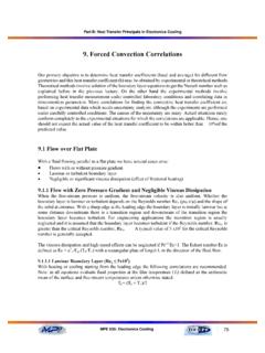
1 Part B: Heat Transfer Principals in Electronics cooling 9. Forced Convection Correlations Our primary objective is to determine heat transfer coefficients (local and average) for different flow geometries and this heat transfer coefficient (h) may be obtained by experimental or theoretical methods. Theoretical methods involve solution of the boundary layer equations to get the Nusselt number such as explained before in the previous lecture. On the other hand the experimental methods involve performing heat transfer measurement under controlled laboratory conditions and correlating data in dimensionless parameters. Many Correlations for finding the convective heat transfer coefficient are based on experimental data which needs uncertainty analysis, although the experiments are performed under carefully controlled conditions.

2 The causes of the uncertainty are many. Actual situations rarely conform completely to the experimental situations for which the Correlations are applicable. Hence, one should not expect the actual value of the heat transfer coefficient to be within better than 10%of the predicted value.. Flow over Flat Plate With a fluid flowing parallel to a flat plate we have several cases arise: Flows with or without pressure gradient Laminar or turbulent boundary layer Negligible or significant viscous dissipation (effect of frictional heating). Flow with Zero Pressure Gradient and Negligible Viscous Dissipation When the free-stream pressure is uniform, the free-stream velocity is also uniform.

3 Whether the boundary layer is laminar or turbulent depends on the Reynolds number ReX ( u x/ ) and the shape of the solid at entrance. With a sharp edge at the leading edge the boundary layer is initially laminar but at some distance downstream there is a transition region and downstream of the transition region the boundary layer becomes turbulent. For engineering applications the transition region is usually neglected and it is assumed that the boundary layer becomes turbulent if the Reynolds number, ReX, is greater than the critical Reynolds number, Recr. A typical value of 5 x105 for the critical Reynolds number is generally accepted.

4 The viscous dissipation and high-speed effects can be neglected if Pr1/2 Ec<1. The Eckert number Ec is defined as Ec = u2 /Cp (TS-T ) with a rectangular plate of length L in the direction of the fluid flow. Laminar Boundary Layer (Rex 5x105). With heating or cooling starting from the leading edge the following Correlations are recommended. Note: in all equations evaluate fluid properties at the film temperature (Tf) defined as the arithmetic mean of the surface and free-stream temperatures unless otherwise stated. Tf = (TS + T )/2. MPE 635: Electronics cooling 75. Part B: Heat Transfer Principals in Electronics cooling Flow with uniform surface temperature (TS = constant).

5 - Local heat transfer coefficient The Nusselt number based on the local convective heat transfer coefficient is expressed as Nu X = f Pr Re 1X/ 2 ( ). The expression of Pr depend on the fluid Prandtl number For liquid metals with very low Prandtl number liquid metals (Pr ). f Pr = Pr 1 / 2. For < Pr < 50. f Pr = Pr 1 / 3. For very large Prandtl number f Pr = Pr 1 / 3. For all Prandtl numbers; Correlations valid developed by Churchill (1976) and Rose (1979) are Re 1x/ 2 Pr 1 / 3 ( ). Nu x = 1/ 4. 2/3.. 1 + . Pr . - Average heat transfer coefficient The average heat transfer coefficient can be evaluated by performing integration along the flat plate length, if Prandtl number is assumed constant along the plate, the integration yields to the following result: Nu x = 2 Nu x ( ).

6 Flow with uniform heat flux (q// = constant). - Local heat transfer coefficient Churchill and Ozoe (1973) recommend the following single correlation for all Prandtl numbers Re1X/ 2 Pr 1 / 2. Nu X = 1/ 4. ( ). Pr 2 / 3 . 1 + .. MPE 635: Electronics cooling 76. Part B: Heat Transfer Principals in Electronics cooling Turbulent Boundary Layer (Rex > 5x105). With heating or cooling starting from the leading edge the following Correlations are recommended. - Local heat transfer coefficient Recr< Rex 107 Nu x = Re 4x / 5 Pr 1 / 3 ( ). Rex >107 Nu x = Re x (ln Re x ) Pr 1 / 3 ( ). Equation is obtained by applying Colburn's j factor in conjunction with the friction factor suggested by Schlichting (1979).

7 With turbulent boundary layers the Correlations for the local convective heat transfer coefficient can be used for both uniform surface temperature and uniform heat flux. - Average heat transfer coefficient If the boundary layer is initially laminar followed by a turbulent boundary layer some times called mixed boundary layer the Following Correlations for < Pr < 60 are suggested: Recr < Rex 107 Nu x = ( Re 4x / 5 871) Pr 1 / 3 ( ). Rex >107 Nu x = [ Re x (ln Re x ) 871] Pr 1 / 3 ( ). Unheated Starting Length Uniform Surface Temperature & Pr > If the plate is not heated or (cooled) from the leading edge where the boundary layer develops from the leading edge until being heated at x = xo as shown in Figure , the Correlations have to be modified.

8 Leading edge . T. xo x Figure Heating starts at x = xo - Local heat transfer coefficient MPE 635: Electronics cooling 77. Part B: Heat Transfer Principals in Electronics cooling Re 1x/ 2 Pr 1 / 3. Laminar flow (Rex < Recr) Nu x = 1/ 3 ( ). xo 3 / 4 . 1 . x . Re 4x / 5 Pr 3 / 5 ( ). Turbulent flow (Rex > Recr) Nu x = 1/ 9. xo 9 / 10.. 1 . x . - Average heat transfer coefficient over the Length (L xo). Laminar flow (ReL < Recr). 2/3. k xo 3 / 4 . h L xo = Re L Pr 1 . 1/ 2 1/ 3. ( ). L xo L . x o . 3/ 4. hx= L. = 2 1 . 1 ( x o / L) L . Evaluate hx=L from Equation Turbulent flow (ReL > Recr). 8/9. x o 9 / 10 . Re L Pr 1.

9 4/5 3/5. k L . h L xo = ( ). L xo 9 / 10. x . 1 o . = . L. hx = L. xo . 1 . L . Evaluate hx=L from Equation Example : Experimental results obtained for heat transfer over a flat plate with zero pressure gradients yields Nu x = Re Pr 1 / 3. Where this correlation is based on x (the distance measured from the leading edge). Calculate the ratio of the average heat transfer coefficient to the local heat transfer coefficient. Schematic: MPE 635: Electronics cooling 78. Part B: Heat Transfer Principals in Electronics cooling x Solution: It is known that hxx Nu x =. k Local heat transfer coefficient k h x = Re Pr 1 / 3. x The average heat transfer coefficient is: Pr 1 / 3 u x.

10 X x 1 1. h x = h x dx = 0 v dx x0 x x x Pr 1 / 3 u . x = dx x v 0. Pr 1/ 3. u . = x x v . = Re Pr 1 / 3. x h = x The ratio of the average heat transfer coefficient to the local heat transfer coefficient is: hx 1. =. h x Example : Air at a temperature of 30 oC and 6 kPa pressure flow with a velocity of 10 m/s over a flat plate m long. Estimate the heat transferred per unit width of the plate needed to maintain its surface at a temperature of 45 oC. Schematic: P =6 kpa u =10 m/s T =30 oC. T S=45 oC. x L= m MPE 635: Electronics cooling 79. Part B: Heat Transfer Principals in Electronics cooling Solution: Properties of the air evaluated at the film temperature Tf = 75/2 = oC.