Transcription of A computer tool for simulation and analysis: the …
1 A computer tool for simulation and analysis : the robotics toolbox for MATLABP eter I. CorkeCSIRO Division of Manufacturing paper introduces, in tutorial form, a Robotics Toolboxfor MATLAB that allowsthe user to easily create and manipulate datatypes fundamental to robotics such as homogeneoustransformations, quaternions and trajectories. Functions provided for arbitrary serial-link ma-nipulators include forward and inverse kinematics, and forward and inverse dynamics. Thecomplete toolbox and documentation is freely available viaanonymous IntroductionMATLAB[1] is a powerful environment for linear algebra and graphical presentation that isavailable on a very wide range of computer platforms. The core functionality can be extended byapplication specific toolboxes. the robotics toolbox provides many functions that are requiredin robotics and addresses areas such as kinematics, dynamics, and trajectory generation.
2 TheToolbox is useful for simulation as well as analyzing results from experiments with real robots,and can be a powerful tool for toolbox is based on a very general method of representingthe kinematics and dynamicsof serial-link manipulators by description matrices. These comprise, in the simplest case, theDenavit and Hartenberg parameters[2] of the robot and can becreated by the user for any serial-link manipulator. A number of examples are provided for wellknown robots such as the Puma560 and the Stanford arm. The manipulator description can beelaborated, by augmenting thematrix, to include link inertial, and motor inertial and frictional parameters. Such matricesprovide a concise means of describing a robot model and may facilitate the sharing of robotmodels across the research community. This would allow simulation results to be comparedin a much more meaningful way than is currently done in the literature.
3 The toolbox alsoprovides functions for manipulating datatypes such as vectors, homogeneous transformationsand unit-quaternions which are necessary to represent 3-dimensional position and routines are generally written in a straightforward, ortextbook, manner for pedagogicalreasons rather than for maximum computational paper is written in a tutorial form and does not require detailed knowledge of MAT-LAB. The examples illustrate both the principal features ofthe toolbox and some elementaryrobotic theory. Section 2 begins by introducing the functions and datatypes used to represent3-dimensional (3D) position and orientation. Section 3 introduces the general matrix repre-sentation of an arbitrary serial-link manipulator and covers kinematics; forward and inversesolutions and the manipulator Jacobians.
4 Section 4 is concerned with the creation of trajecto-ries in configuration or Cartesian space. Section 5 extends the general matrix representation toinclude manipulator rigid-body and motor dynamics, and describes functions for forward andinverse manipulator dynamics. Details on how to obtain the package are given in Section Representing 3D translation and orientationIn Cartesian coordinates translation may be represented bya position vector,Ap, with respectto the origin of coordinate frameAand wherep 3. IfAis not given the world coordinateframe is assumed. Many representations of 3D orientation have been proposed[3] but the mostcommonly used in robotics are orthonormal rotation matrices and unit-quaternions. The homo-geneous transformation is a 4 4 matrix which represents translation and orientation and canbe compounded simply by matrix multiplication.
5 Such a matrix representation is well matchedto MATLAB s powerful capability for matrix manipulation. Homogeneous transformationsT=[Rp0 0 0 1](1)describe the relationships between Cartesian coordinate frames in terms of a Cartesian trans-lation,p, and orientation. expressed as an orthonormal rotation matrix,Ris a 3 3. A ho-mogeneous transformation representing a pure translationof m in the X-direction is createdby>> T = transl( , , )T = 0 0 0 00 0 00 0 0 a rotation of 90 about the Y-axis by>> T = roty(pi/2)T = 0 00 0 0 00 0 0 transforms may be concatenated by multiplication, forinstance,>> T = transl( , , ) * roty(pi/2) * rotz(-pi/2)T = 0 00 0 0 resulting transformation may be interpreted as a new coordinate frame whose X-, Y- andZ-axes are parallel to unit vectors given by the first three columns ofT.
6 That is, the new X-axisis anti-parallel to the world Y-axis, and so on. The orientation of the new coordinate frame maybe expressed in terms of Euler angles>> tr2eul(T)ans =0 units of radians, or roll/pitch/yaw angles>> rpy = tr2rpy(T)rpy = transforms can be generated from Euler or roll/pitch/yaw angles, or by rotationabout an arbitrary vector using the functionseul2tr(),rpy2tr(),rotvec() can also be represented by a quaternion[3], which will be denoted here byq= [s,v](2)wheresis a scalar andv 3. A unit-quaternion has unit magnitude, that is,s2+|v|2=1in which cases=sin /2, andqcan be considered as a rotation of about the vectorv. Therotational component of a homogeneous transform can be converted to a unit-quaternion>> q = tr2q(T)q = indicates that the compounded transformation is equivalent to a rotation of rad aboutthe vector[ 1 1 1].
7 Quaternions can be compounded ( multiplied ) by the functionqmul().Quaternions offer several advantages over homogeneous transformations such as reduced arith-metic cost when compounding rotations, simpler rotationalinterpolation, and less need for nor-malization to counter the effects of numerical roundoff. Torepresent translation as well asrotation a quaternion/vector pair can be employed[3] but such a composite type is not yet sup-ported by this KinematicsForward kinematics is the problem of solving the Cartesian position and orientation of theend-effector given knowledge of the kinematic structure and the joint coordinates. The kine-matic structure of a serial-link manipulator can be succinctly described in terms of Denavit-Hartenberg parameters[2]. Within the toolbox the manipulator s kinematics are representedin a general way by adhmatrix which is given as the first argument to toolbox kinematicfunctions.
8 Thedhmatrix describes the kinematics of a manipulator using the standard Denavit-Hartenberg conventions, where each row represents one linkof the manipulator and the columnsare assigned according to the following table:Column SymbolDescription1 ilink twist angle (rad)2 Ailink offset distance3 ilink rotation angle (rad)4 Dilink length5 ioptional joint type; 0 for revolute, non-zero for 1: Visualization of Puma robot at zero joint angle pose created byplotbot(p560,qz).If the last column is not given, toolbox functions assume that the manipulator is an n-axis manipulatordhis ann 4 orn 5 matrix. Joint angles are represented byn-element row the example of a Puma 560 manipulator, a common laboratory robot. The kine-matics may be defined by thepuma560command which creates a kinematic description matrixp560in the workspace using standard Denavit-Hartenberg conventions, and the particular frameassignments of Paul and Zhang[4].
9 It also creates workspacevariables that define special jointangle poses:qzfor all zero joint angles,qrfor the READY position andqstretchfor a fullyextended arm horizontal pose. The forward kinematics may becomputed for the zero anglepose>> puma560 % define puma kinematic matrix p560>> fkine(p560, qz)ans = 0 0 0 0 0 0 returns the homogeneous transform corresponding to the last link of the translation, given by the last column, is in the same dimensional units as theAiandDidatain thedhmatrix, in this case metres. This pose can be visualized by>> plotbot(p560, qz);which produces the 3-D plot shown in Figure 1. The drawn line segments do not necessarilycorrespond to robot links, but join the origins of sequential link coordinate frames.
10 This simpleapproach eliminates the need for detailed robot geometry data. A small right-handed coordinateframe is drawn on the end of the robot to show the wrist orientation. The X-, Y- and Z-axes arerepresented by the colors red, green and blue kinematics is the problem of finding the robot joint coordinates, given a homoge-neous transform representing the pose of the is very useful when the path isplanned in Cartesian space, for instance a straight line path as shown later. First generate thetransform corresponding to a particular joint coordinate,>> q = [0 -pi/4 -pi/4 0 pi/8 0]q =0 0 0>> T = fkine(p560, q);and then find the corresponding joint angles usingikine()>> qi = ikine(p560, T)qi = compares well with the original inverse kinematic procedure for any specific robot can bederived symbolically[2] andcommonly an efficient closed-form solution can be the toolbox is given onlya generalized description of the manipulator in terms of kinematic parameters so an iterativenumerical solution must be used.