Transcription of A Practical Guide to Wavelet Analysis
1 61 Bulletin of the American Meteorological Society1. IntroductionWavelet Analysis is becoming a common tool foranalyzing localized variations of power within a timeseries. By decomposing a time series into time fre-quency space, one is able to determine both the domi-nant modes of variability and how those modes varyin time . The Wavelet transform has been used for nu-merous studies in geophysics, including tropical con-vection (Weng and Lau 1994), the El Ni o SouthernOscillation (ENSO; Gu and Philander 1995; Wang andWang 1996), atmospheric cold fronts (Gamage andBlumen 1993), central England temperature (Baliunaset al. 1997), the dispersion of ocean waves (Meyers etal. 1993), wave growth and breaking (Liu 1994), andcoherent structures in turbulent flows (Farge 1992). Acomplete description of geophysical applications canbe found in Foufoula-Georgiou and Kumar (1995),while a theoretical treatment of Wavelet Analysis isgiven in Daubechies (1992).
2 Unfortunately, many studies using Wavelet analy-sis have suffered from an apparent lack of quantita-tive results. The Wavelet transform has been regardedby many as an interesting diversion that produces col-orful pictures, yet purely qualitative results. This mis-conception is in some sense the fault of Wavelet analy-sis itself, as it involves a transform from a one-dimen-sional time series (or frequency spectrum) to a diffusetwo-dimensional time frequency image. This diffuse-ness has been exacerbated by the use of arbitrary nor-malizations and the lack of statistical significance Lau and Weng (1995), an excellent introductionto Wavelet Analysis is provided. Their paper, however,did not provide all of the essential details necessaryfor Wavelet Analysis and avoided the issue of statisti-cal purpose of this paper is to provide an easy-to-use Wavelet Analysis toolkit, including statistical sig-nificance testing.
3 The consistent use of examples ofA Practical Guide toWavelet AnalysisChristopher Torrence and Gilbert P. CompoProgram in Atmospheric and Oceanic Sciences, University of Colorado, Boulder, ColoradoABSTRACTA Practical step-by-step Guide to Wavelet Analysis is given, with examples taken from time series of the El Ni o Southern Oscillation (ENSO). The Guide includes a comparison to the windowed Fourier transform, the choice of anappropriate Wavelet basis function, edge effects due to finite-length time series , and the relationship between waveletscale and Fourier frequency. New statistical significance tests for Wavelet power spectra are developed by deriving theo-retical Wavelet spectra for white and red noise processes and using these to establish significance levels and confidenceintervals. It is shown that smoothing in time or scale can be used to increase the confidence of the Wavelet formulas are given for the effect of smoothing on significance levels and confidence intervals.
4 Extensions towavelet Analysis such as filtering, the power Hovm ller, cross- Wavelet spectra, and coherence are statistical significance tests are used to give a quantitative measure of changes in ENSO variance on interdecadaltimescales. Using new datasets that extend back to 1871, the Ni o3 sea surface temperature and the Southern Oscilla-tion index show significantly higher power during 1880 1920 and 1960 90, and lower power during 1920 60, as wellas a possible 15-yr modulation of variance. The power Hovm ller of sea level pressure shows significant variations in2 8-yr Wavelet power in both longitude and author address: Dr. Christopher Torrence, Ad-vanced Study Program, National Center for Atmospheric Re-search, Box 3000, Boulder, CO : final form 20 October 1997. 1998 American Meteorological Society62 Vol.
5 79, No. 1, January 1998 ENSO provides a substantive addition tothe ENSO literature. In particular, thestatistical significance testing allowsgreater confidence in the previous wave-let-based ENSO results of Wang andWang (1996). The use of new datasetswith longer time series permits a morerobust classification of interdecadalchanges in ENSO first section describes the datasetsused for the examples. Section 3 de-scribes the method of Wavelet analysisusing discrete notation. This includes adiscussion of the inherent limitations ofthe windowed Fourier transform (WFT),the definition of the Wavelet transform,the choice of a Wavelet basis function,edge effects due to finite-length time se- ries , the relationship between waveletscale and Fourier period, and time seriesreconstruction.
6 Section 4 presents thetheoretical Wavelet spectra for bothwhite-noise and red-noise theoretical spectra are compared toMonte Carlo results and are used to es-tablish significance levels and confi-dence intervals for the Wavelet powerspectrum. Section 5 describes time orscale averaging to increase significancelevels and confidence intervals. Section6 describes other Wavelet applicationssuch as filtering, the power Hovm ller,cross- Wavelet spectra, and Wavelet co-herence. The summary contains a step-by-step Guide to Wavelet DataSeveral time series will be used for examples ofwavelet Analysis . These include the Ni o3 sea surfacetemperature (SST) used as a measure of the amplitudeof the El Ni o Southern Oscillation (ENSO). TheNi o3 SST index is defined as the seasonal SST av-eraged over the central Pacific (5 S 5 N, 90 150 W).
7 Data for 1871 1996 are from an area aver-age of the Meteorological Office (Rayner et al. 1996), while data for January June 1997are from the Climate Prediction Center (CPC) opti-mally interpolated Ni o3 SST index (courtesy of at CPC, NOAA). The seasonal means for theentire record have been removed to define an anomalytime series . The Ni o3 SST is shown in the top plotof Fig. sea level pressure (SLP) data is from theUKMO/CSIRO historical (courtesy of and T. Basnett, Hadley Centre for Climate Pre-diction and Research, UKMO). The data is on a 5 global grid, with monthly resolution from January1871 to December 1994. Anomaly time series havebeen constructed by removing the first three harmon-ics of the annual cycle (periods of , , days) using a least-squares Southern Oscillation index is derived from and is defined as the seasonally averagedpressure difference between the eastern Pacific (20 S,150 W) and the western Pacific (10 S, 130 E).
8 1880190019201940196019802000-2-10123 (oC)a. NINO3 SST 1880190019201940196019802000 time (year)1248163264 Period (years) (years) b. Morlet1880190019201940196019802000 time (year)12481632 Period (years) (years) c. DOGFIG. 1. (a) The Ni o3 SST time series used for the Wavelet Analysis . (b) Thelocal Wavelet power spectrum of (a) using the Morlet Wavelet , normalized by 1/ 2 ( 2 = C2). The left axis is the Fourier period (in yr) corresponding to thewavelet scale on the right axis. The bottom axis is time (yr). The shaded contoursare at normalized variances of 1, 2, 5, and 10. The thick contour encloses regionsof greater than 95% confidence for a red-noise process with a lag-1 coefficient Cross-hatched regions on either end indicate the cone of influence, whereedge effects become important. (c) Same as (b) but using the real-valued Mexicanhat Wavelet (derivative of a Gaussian; DOG m = 2).
9 The shaded contour is atnormalized variance of of the American Meteorological Society3. Wavelet analysisThis section describes the method of Wavelet analy-sis, includes a discussion of different Wavelet func-tions, and gives details for the Analysis of the waveletpower spectrum. Results in this section are adapted todiscrete notation from the continuous formulas givenin Daubechies (1990). Practical details in applyingwavelet Analysis are taken from Farge (1992), Wengand Lau (1994), and Meyers et al. (1993). Each sec-tion is illustrated with examples using the Ni o3 Windowed Fourier transformThe WFT represents one Analysis tool for extract-ing local-frequency information from a signal. TheFourier transform is performed on a sliding segmentof length T from a time series of time step t and totallength N t, thus returning frequencies from T 1 to(2 t) 1 at each time step.
10 The segments can be win-dowed with an arbitrary function such as a boxcar (nosmoothing) or a Gaussian window (Kaiser 1994).As discussed by Kaiser (1994), the WFT representsan inaccurate and inefficient method of time fre-quency localization, as it imposes a scale or responseinterval T into the Analysis . The inaccuracy arisesfrom the aliasing of high- and low-frequency compo-nents that do not fall within the frequency range of thewindow. The inefficiency comes from the T/(2 t) fre-quencies, which must be analyzed at each time step,regardless of the window size or the dominant frequen-cies present. In addition, several window lengths mustusually be analyzed to determine the most appropri-ate choice. For analyses where a predetermined scal-ing may not be appropriate because of a wide rangeof dominant frequencies, a method of time frequencylocalization that is scale independent, such as wave-let Analysis , should be Wavelet transformThe Wavelet transform can be used to analyze timeseries that contain nonstationary power at many dif-ferent frequencies (Daubechies 1990).