A Tutorial on Principal Component Analysis

1 A Tutorial on Principal Component AnalysisJonathon Shlens Systems Neurobiology Laboratory,Salk Insitute for Biological StudiesLa Jolla, CA 92037 andInstitute for Nonlinear Science,University of California,San DiegoLa Jolla, CA 92093-0402(Dated: December 10, 2005; Version 2) Principal Component Analysis (PCA) is a mainstay of modern data Analysis - a black box thatis widely used but poorly understood. The goal of this paper is to dispel the magic behind thisblack box. This Tutorial focuses on building a solid intuition for how and why Principal componentanalysis works; furthermore, it crystallizes this knowledge by deriving from simple intuitions, themathematics behindPCA. This Tutorial does not shy away from explaining the ideas informally,nor does it shy away from the mathematics. The hope is that by addressing both aspects, readersof all levels will be able to gain a better understanding ofPCAas well as the when, the how andthe why of applying this INTRODUCTIONP rincipal Component Analysis (PCA) has been calledone of the most valuable results from applied linear used abundantly in all forms of Analysis -from neuroscience to computer graphics - because it is asimple, non-parametric method of extracting relevant in-formation from confusing data sets.

2 With minimal addi-tional effortPCAprovides a roadmap for how to reducea complex data set to a lower dimension to reveal thesometimes hidden, simplified structure that often under-lie goal of this Tutorial is to provide both an intuitivefeel forPCA, and a thorough discussion of this will begin with a simple example and provide an intu-itive explanation of the goal ofPCA. We will continue byadding mathematical rigor to place it within the frame-work of linear algebra to provide an explicit solution. Wewill see how and whyPCAis intimately related to themathematical technique of singular value decomposition(SVD). This understanding will lead us to a prescriptionfor how to applyPCAin the real world. We will discussboth the assumptions behind this technique as well aspossible extensions to overcome these discussion and explanations in this paper are infor-mal in the spirit of a Tutorial . The goal of this paper is toeducate.

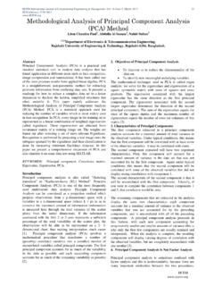
3 Occasionally, rigorous mathematical proofs arenecessary although relegated to the Appendix. Althoughnot as vital to the Tutorial , the proofs are presented forthe adventurous reader who desires a more complete un-derstanding of the math. The only assumption is that thereader has a working knowledge of linear algebra. Pleasefeel free to contact me with any suggestions, correctionsor comments. Electronic MOTIVATION: A TOY EXAMPLEHere is the perspective: we are an experimenter. Weare trying to understand some phenomenon by measur-ing various quantities ( spectra, voltages, velocities,etc.) in our system. Unfortunately, we can not figure outwhat is happening because the data appears clouded, un-clear and even redundant. This is not a trivial problem,but rather a fundamental obstacle in empirical abound from complex systems such as neu-roscience, photometry, meteorology and oceanography -the number of variables to measure can be unwieldy andat times evendeceptive, because the underlying relation-ships can often be quite for example a simple toy problem from physicsdiagrammed in Figure 1.

4 Pretend we are studying themotion of the physicist s ideal spring. This system con-sists of a ball of massmattached to amassless, friction-lessspring. The ball is released a small distance awayfrom equilibrium ( the spring is stretched). Becausethe spring is ideal, it oscillates indefinitely along thex-axis about its equilibrium at a set is a standard problem in physics in which the mo-tion along thexdirection is solved by an explicit functionof time. In other words, the underlying dynamics can beexpressed as a function of a single , being ignorant experimenters we do not knowany of this. We do not know which, let alone howmany, axes and dimensions are important to , we decide to measure the ball s position in athree-dimensional space (since we live in a three dimen-sional world). Specifically, we place three movie camerasaround our system of interest. At 200 Hz each moviecamera records an image indicating a two dimensionalposition of the ball (a projection).

5 Unfortunately, be-cause of our ignorance, we do not even know what arethereal x , y and z axes, so we choose three cam-era axes{~a,~b,~c}at some arbitrary angles with respectto the system. The angles between our measurements2 FIG. 1 A diagram of the toy not even be 90o! Now, we record with the camerasfor several minutes. The big question remains:how dowe get from this data set to a simple equation ofx?We know a-priori that if we were smart experimenters,we would have just measured the position along thex-axis with one camera. But this is not what happens in thereal world. We often do not know which measurementsbest reflect the dynamics of our system in question. Fur-thermore, we sometimes record more dimensions than weactually need!Also, we have to deal with that pesky, real-world prob-lem ofnoise. In the toy example this means that weneed to deal with air, imperfect cameras or even frictionin a less-than-ideal spring.

6 Noise contaminates our dataset only serving to obfuscate the dynamics example is the challenge experimenters face will refer to this example as we delve further into ab-stract concepts. Hopefully, by the end of this paper wewill have a good understanding of how to systematicallyextractxusing Principal Component FRAMEWORK: CHANGE OF BASISThe goal of Principal Component Analysis is to computethe most meaningfulbasisto re-express a noisy data hope is that this new basis will filter out the noiseand reveal hidden structure. In the example of the spring,the explicit goal ofPCAis to determine: the dynamicsare along thex-axis. In other words, the goal ofPCAis to determine that x- the unit basis vector along thex-axis - is the important dimension. Determining thisfact allows an experimenter to discern which dynamicsare important, which are just redundant and which arejust A Naive BasisWith a more precise definition of our goal, we needa more precise definition of our data as well.

7 We treatevery time sample (or experimental trial) as an individualsample in our data set. At each time sample we recorda set of data consisting of multiple measurements ( , position, etc.). In our data set, at one pointin time, cameraArecords a corresponding ball position(xA, yA). One sample or trial can then be expressed as a6 dimensional column vector~X= xAyAxByBxCyC where each camera contributes a 2-dimensional projec-tion of the ball s position to the entire vector~X. If werecord the ball s position for 10 minutes at 120 Hz, thenwe have recorded 10 60 120 = 72000 of these this concrete example, let us recast this problemin abstract terms. Each sample~Xis anm-dimensionalvector, wheremis the number of measurement , every sample is a vector that lies in anm-dimensionalvector spacespanned by some orthonormalbasis. From linear algebra we know that all measurementvectors form a linear combination of this set of unit lengthbasis vectors.

8 What is this orthonormal basis?This question is usually a tacit assumption often over-looked. Pretend we gathered our toy example data above,but only looked at cameraA. What is an orthonormal ba-sis for (xA, yA)? A naive choice would be{(1,0),(0,1)},but why select this basis over{( 22, 22),( 22, 22)}orany other arbitrary rotation? The reason is that thenaive basis reflects the method we gathered the we record the position (2,2). We didnotrecord2 2 in the ( 22, 22) direction and 0 in the perpindicu-lar direction. Rather, we recorded the position (2,2) onour camera meaning 2 unitsupand 2 units to theleftin our camera window. Thus our naive basis reflects themethod we measured our do we express this naive basis in linear algebra?In the two dimensional case,{(1,0),(0,1)}can be recastas individual row vectors. A matrix constructed out ofthese row vectors is the 2 2 identity matrixI. We cangeneralize this to them-dimensional case by constructinganm midentity matrixB= = 1 0 00 1 0 1 =Iwhere eachrowis an orthornormal basis vectorbiwithmcomponents.

9 We can consider our naive basis as theeffective starting point. All of our data has been recordedin this basis and thus it can be trivially expressed as alinear combination of{bi}.3B. Change of BasisWith this rigor we may now state more precisely whatPCAasks:Is there another basis, which is a linear com-bination of the original basis, that best re-expresses ourdata set?A close reader might have noticed the conspicuous ad-dition of the wordlinear. Indeed,PCAmakes one strin-gent but powerful assumption:linearity. Linearity vastlysimplifies the problem by (1) restricting the set of poten-tial bases, and (2) formalizing the implicit assumption ofcontinuity in a data this assumptionPCAis now limited to re-expressing the data as alinear combinationof its ba-sis vectors. LetXbe the original data set, where eachcolumnis a single sample (or moment in time) of our dataset ( ~X). In the toy exampleXis anm nmatrixwherem= 6 andn= 72000.

10 LetYbe anotherm nmatrix related by a linear theoriginal recorded data set andYis a re-representation ofthat data (1)Also let us define the following piare therowsofP xiare thecolumnsofX(or individual~X). yiare 1 represents achange of basisand thus can havemany a matrix that Geometrically,Pis a rotation and a stretch whichagain The rows ofP,{p1, .. ,pm}, are a set of new basisvectors for expressing latter interpretation is not obvious but can be seenby writing out the explicit dot products x1 xn Y= p1 x1 p1 x1 pm xn 1A subtle point it is, but we have already assumed linearity byimplicitly stating that the data set even characterizes thedy-namics of the system. In other words, we are already relying onthe superposition Principal of linearity to believe that the dataprovides an ability to interpolate between individual datapoints2In this sectionxiandyiarecolumnvectors, but be all other can note the form of each column p1 xi We recognize that each coefficient ofyiis a dot-productofxiwith the corresponding row inP.