Transcription of An Introduction in Structural Equation Modeling
1 Introduction Structural Equation Modeling1 Family Science Review, 11, Introduction to Structural Equation HoxUniversity of Amsterdam/Utrecht BechgerCITO, ArnhemAbstract This article presents a short and non-technical Introduction to StructuralEquation Modeling or SEM. SEM is a powerful technique that can combine complex pathmodels with latent variables (factors). Using SEM, researchers can specify confirmatoryfactor analysis models, regression models, and complex path models. We present thebasic elements of a Structural Equation model, introduce the estimation technique, whichis most often maximum Likelihood (ML), and discuss some problems concerning theassessment and improvement of the model fit, and model extensions to multigroupproblems including factor means. Finally, we discuss some of the software, and list usefulhandbooks and Internet is Structural Equation Modeling ?
2 Structural Equation Modeling , or SEM, is a very general statistical Modeling technique,which is widely used in the behavioral sciences. It can be viewed as a combination offactor analysis and regression or path analysis. The interest in SEM is often on theoreticalconstructs, which are represented by the latent factors. The relationships between thetheoretical constructs are represented by regression or path coefficients between thefactors. The Structural Equation model implies a structure for the covariances between theobserved variables, which provides the alternative name covariance structure , the model can be extended to include means of observed variables or factors inthe model, which makes covariance structure Modeling a less accurate name. Manyresearchers will simply think of these models as Lisrel-models, which is also lessaccurate.
3 LISREL is an abbreviation of LInear Structural RELations, and the name used byJ reskog for one of the first and most popular SEM programs. Nowadays structuralequation models need not be linear, and the possibilities of SEM extend well beyond theoriginal Lisrel program. Browne (1993), for instance, discusses the possibility to fitnonlinear Equation Modeling provides a very general and convenient frameworkfor statistical analysis that includes several traditional multivariate procedures, forexample factor analysis, regression analysis, discriminant analysis, and canonicalcorrelation, as special cases. Structural Equation models are often visualized by agraphical path diagram. The statistical model is usually represented in a set of matrixequations. In the early seventies, when this technique was first introduced in social andbehavioral research, the software usually required setups that specify the model in termsof these matrices.
4 Thus, researchers had to distill the matrix representation from the pathdiagram, and provide the software with a series of matrices for the different sets of 1 Note: The authors thank Alexander Vazsonyi and three anonymous reviewers for their comments on aprevious version. We thank Annemarie Meijer for her permission to use the quality of sleep Structural Equation Modeling2parameters, such as factor loadings and regression coefficients. A recent development issoftware that allows the researchers to specify the model directly as a path diagram. Thisworks well with simple problems, but may get tedious with more complicated that reason, current SEM software still supports the command- or matrix-style modelspecifications review provides a brief and non-technical review of the basic issues involvedin SEM, including issues of estimation, model fit, and statistical assumptions.
5 We includea list of available software, introductory books, and useful Internet of SEM-ModelsIn this section, we set the stage by discussing examples of a confirmatory factor analysis,regression analysis, and a general Structural Equation model with latent Equation Modeling has its roots in path analysis, which was invented bythe geneticist Sewall Wright (Wright, 1921). It is still customary to start a SEM analysisby drawing a path diagram. A path diagram consists of boxes and circles, which areconnected by arrows. In Wright s notation, observed (or measured) variables arerepresented by a rectangle or square box, and latent (or unmeasured) factors by a circle orellipse. Single headed arrows or paths are used to define causal relationships in themodel, with the variable at the tail of the arrow causing the variable at the point.
6 Doubleheaded arrows indicate covariances or correlations, without a causal , the single headed arrows or paths represent regression coefficients, anddouble-headed arrows covariances. Extensions of this notation have been developed torepresent variances and means (cf. McArdle, 1996). The first example in Figure 1 is arepresentation of a confirmatory factor analysis model, with six observed variables andtwo Factor AnalysisThe model in Figure 1 is a confirmatory factor model for data collected by Holzinger andSwineford, extracted from the AMOS manual (Arbucle, 1997, p. 375, see also J reskog &S rbom, 1989, p. 247). The data are the scores of 73 girls on six intelligence tests. Thereare two hypothesized intelligence factors, a verbal and a spatial ability factor, which aredrawn as latent factors which are assumed to cause the variation and covariation betweenthe six observed variables.
7 There is a double-headed arrow between the two factors,which indicates that we assume that the two factors are correlated. The arrows from thefactors to the variables represent linear regression coefficients or factor loadings . We donot assume that the latent factors completely explain the observed variation; eachobserved variable is associated with a residual error term, which is also unmeasured anddepicted by a Structural Equation Modeling3spatialvisperccubeslozengesword meanparagraphsentencee_ve_ce_le_pe_se_wv erbal11111111 Figure 1. Confirmatory Factor analysis;Holzinger and Swineford analysis assumes that the covariances between a set of observed variables can beexplained by a smaller number of underlying latent factors. In exploratory factor analysis,we proceed as if we have no hypothesis about the number of latent factors and therelations between the latent factors and the observed variables.
8 Statistical procedures areused to estimate the number of underlying factors, and to estimate the factor loadings. Inexploratory factor analysis, the model is arbitrary: all variables load on all , a transformation method such as Varimax rotation is used to improve theinterpretation of the results. In contrast, the path diagram in Figure 1 represents a clearhypothesis about the factor structure. Models of this kind are called restricted orconfirmatory factor analysis (CFA) models. In Structural Equation Modeling , theconfirmatory factor model is imposed on the data. In this case, the purpose of structuralequation Modeling is twofold. First, it aims to obtain estimates of the parameters of themodel, the factor loadings, the variances and covariances of the factor, and theresidual error variances of the observed variables.
9 The second purpose is to assess the fitof the model, to assess whether the model itself provides a good fit to the data. Wewill deal with these issues in more detail , some of the factor loadings are constrained or fixed to be zero. InFigure 1, the absence of arrows going from the verbal factor to visperc, cubes and lozenges, means that the corresponding loadings in the factor matrix are fixed to , the loadings of paragraph, sentence and wordmean on the spatial factorare also fixed to zero. The factor model in Figure 1 shows a perfect simple structure: eachvariable loads on one factor only. Confirmative factor analysis can specify such astructure exactly, and test whether it is plausible, while explorative factor analysis canonly approximate such simple structures by each factor, we also must fix one loading to one.
10 This is needed to give thelatent factor an interpretable scale. If we do not fix one factor loading to one for (or toanother number not equal to zero), the scale of the latent factor is undetermined. For eachlatent factor, we can estimate the loadings given a fixed variance for the latent factor, Introduction Structural Equation Modeling4which standardizes the scale of the factor to a Z-score, or we can estimate the factorvariance given at least one fixed loading. Since the loadings are a function of the varianceof the latent factor, and the variance of the latent factor is a function of the loadings, wecannot simultaneously estimate unique values for all of these. Thus, one solution here isto fix the variance of all factors to one, and estimate all factor loadings. In SEM, it ismore customary to use the other solution, which is to fix one loading for each factor toone, and estimate the factor variances.