Transcription of An Introduction to Mathematical Optimal Control Theory ...
1 An Introduction to MathematicalOptimal Control TheoryVersion C. EvansDepartment of MathematicsUniversity of California, BerkeleyChapter 1: IntroductionChapter 2: Controllability, bang-bang principleChapter 3: Linear time- Optimal controlChapter 4: The Pontryagin Maximum PrincipleChapter 5: Dynamic programmingChapter 6: Game theoryChapter 7: Introduction to stochastic Control theoryAppendix: Proofs of the Pontryagin Maximum PrincipleExercisesReferences1 PREFACET hese notes build upon a course I taught at the University of Maryland duringthe fall of 1983.
2 My great thanks go to Martino Bardi, who tookcareful notes,saved them all these years and recently mailed them to me. Faye Yeager typed uphis notes into a first draft of these lectures as they now appear. Scott Armstrongread over the notes and suggested many improvements: thanks, Scott. StephenMoye of the American Math Society helped me a lot with AMSTeX versus LaTeXissues. My thanks also to Atilla Yilmaz for spotting lots of typos and errors, whichI have have radically modified much of the notation (to be consistent with my otherwritings), updated the references, added several new examples, and provided a proofof the Pontryagin Maximum Principle.
3 As this is a course for undergraduates, I havedispensed in certain proofs with various measurability andcontinuity issues, and ascompensation have added various critiques as to the lack of total current version of the notes is not yet complete, but meets I think theusual high standards for material posted on the internet. Please email me with any corrections or 1: The basic Some A geometric THE BASIC open our discussion by considering an ordinary differentialequation (ODE) having the form( ) x(t) =f(x(t))(t >0)x(0) = are here given the initial pointx0 Rnand the functionf:Rn un-known is the curvex: [0, ) Rn, which we interpret as the dynamical evolutionof the state of some system.]
4 CONTROLLED generalize a bit and suppose now thatfdepends also upon some Control parameters belonging to a setA Rm; so thatf:Rn A if we select some valuea Aand consider the correspondingdynamics: x(t) =f(x(t),a)(t >0)x(0) =x0,we obtain the evolution of our system when the parameter is constantly set to next possibility is that we change the value of the parameter as the systemevolves. For instance, suppose we define the function : [0, ) Athis way: (t) = a10 t t1a2t1< t t2a3t2< t times 0< t1< t2< parameter valuesa1,a2,a3, A; and we thensolve the dynamical equation( ) x(t) =f(x(t), (t))(t >0)x(0) = picture illustrates the resulting evolution.]
5 The pointis that the system maybehave quite differently as we change the Control = a1t1t2t3trajectory of ODEtime = a3 = a2 = a4 Controlled dynamicsMore generally, we call a function : [0, ) Aacontrol. Corresponding toeach Control , we consider the ODE(ODE) x(t) =f(x(t), (t))(t >0)x(0) =x0,and regard the trajectoryx( ) as the correspondingresponseof the (i) We will writef(x,a) = f1(x,a)..fn(x,a) to display the components off, and similarly putx(t) = x1(t)..xn(t) .We will therefore write vectors as columns in these notes anduse boldface forvector-valued functions, the components of which have superscripts.]
6 (ii) We also introduceA={ : [0, ) A| ( ) measurable}4to denote the collection of alladmissible controls, where (t) = 1(t).. m(t) .Note very carefully that our solutionx( ) of (ODE) depends upon ( ) and the initialcondition. Consequently our notation would be more precise, but more complicated,if we were to writex( ) =x( , ( ),x0),displaying the dependence of the responsex( ) upon the Control and the initialvalue. overall task will be to determine what is the best Control forour system. For this we need to specify a specific payoff (or reward) criterion.]
7 Letus define thepayoff functional(P)P[ ( )] :=ZT0r(x(t), (t))dt+g(x(T)),wherex( ) solves (ODE) for the Control ( ). Herer:Rn A Randg:Rn Rare given, and we callrtherunning payoffandgtheterminal payoff. The terminaltimeT >0 is given as BASIC aim is to find a Control ( ), whichmaximizesthe payoff. In other words, we wantP[ ( )] P[ ( )]for all controls ( ) A. Such a Control ( ) is task presents us with these Mathematical issues:(i) Does an Optimal Control exist?(ii) How can we characterize an Optimal Control mathematically?
8 (iii) How can we construct an Optimal Control ?These turn out to be sometimes subtle problems, as the following collection ofexamples EXAMPLESEXAMPLE 1: Control of production AND we own, say, a factory whose output we can Control . Let us begin toconstruct a Mathematical model by settingx(t) = amount of output produced at timet suppose that we consume some fraction of our output at eachtime, and likewisecan reinvest the remaining fraction. Let us denote (t) = fraction of output reinvested at timet will be our Control , and is subject to the obvious constraint that0 (t) 1 for each timet such a Control , the corresponding dynamics are provided by the ODE x(t) =k (t)x(t)x(0) = constantk >0 modelling the growth rate of our reinvestment.
9 Let us take as apayoff functionalP[ ( )] =ZT0(1 (t))x(t) meaning is that we want to maximize our total consumptionof the output, ourconsumption at a given timetbeing (1 (t))x(t). This model fits into our generalframework forn=m= 1, once we putA= [0,1], f(x,a) =kax, r(x,a) = (1 a)x, g * * = 1 * = 0A bang-bang controlAs we will see later in , an Optimal Control ( ) is given by (t) = 1 if 0 t t 0 ift < t Tfor an appropriateswitching time0 t T. In other words, we should reinvestall the output (and therefore consume nothing) up until timet , and afterwards, weshould consume everything (and therefore reinvest nothing).
10 The switchover timet will have to be determined. We call ( ) abang bangcontrol. EXAMPLE 2: REPRODUCTIVE STATEGIES IN SOCIAL INSECTS6 The next example is from Chapter 2 of the bookCaste and Ecology in SocialInsects, by G. Oster and E. O. Wilson [O-W]. We attempt to model how socialinsects, say a population of bees, determine the makeup of their us writeTfor the length of the season, and introduce the variablesw(t) = number of workers at timetq(t) = number of queens (t) = fraction of colony effort devoted to increasing work forceThe Control is constrained by our requiring that0 (t) continue to model by introducing dynamics for the numbersof workers andthe number of queens.