Transcription of An Introduction to the Boundary Element Method (BEM)
1 1An Introduction to the Boundary Element Method (BEM) and Its Applications in EngineeringYijun LiuUpdated: October 20, 2018 Available at: Boundary Element Method (BEM)nnn Boundary Element methodapplies surface elements on the Boundary of a 3-D domain and line elements on the Boundary of a 2-D domain. The number of elements is O(n2) as compared to O(n3) in other domain based methods (n= number of elements needed per dimension). BEM is good for problems with complicated geometries, stress concentration problems, infinite domain problems, wave propagation problems, and many others. finite Element methodcan solve a model with 1 million DOFs on a PC with 1 GB RAM.
2 Fast multipole BEMcan also solve a model with 1 million DOFs on a PC with 1 GB RAM. However, these DOFs are on the boundaryof the model only, which would require 1billion DOFs for thecorresponding domain Comparison of the FEM and BEM- An Engine Block Model Heat conduction of a V6 engine model is studied. ANSYS is used in the FEM study. Fast multipole BEM is used in the BEM study. A linear temperature distribution is applied on the six cylindrical surfacesFEM (363,180 volume elements )BEM (42,169 surface elements )4 FEM Results(50 min.)BEM Results(16 min.)A Comparison of the FEM and BEMwith An Engine Block Model (Cont.)
3 5 Two Different Routes in Computational MechanicsEngineering ProblemsMathematical ModelsDifferential Equation (ODE/PDE) FormulationsBoundary Integral Equation (BIE) FormulationsAnalytical SolutionsAnalytical SolutionsNumerical SolutionsNumerical SolutionsFDMFEMEFMO thersBEMO thersBNM6A Brief History of the BEMBEM emergedin 1980 s ..Integral equations(Fredholm, 1903)Modern numerical solutionsof BIEs (in early 1960 s)Jaswon and Symm(1963) 2D Potential ProblemsFrank J. Rizzo(Dissertation in 1964 at TAM of UIUC, paper published in 1967) 2D Elasticity ProblemsT. A. Cruse and F. J. Rizzo(1968) 2D elastodynamicsP.
4 K. Banerjee(1975) Coined the name Boundary Element Method Frank J. RizzoU WashingtonU KentuckyIowa State UU IllinoisP. K. BanerjeeU Wales, UKSUNY - BuffaloSubrata MukherjeeCornell UThomas A. CruseBoeingCMUP ratt & WhitneySwRIVanderbilt UAFRLP ioneers in the BIE/BEM Research in the Others8 Pioneers in Early BIE/BEM Research in China .. OthersMy Earlier BEM Research Analysis of Large-Deflection of Elastic PlatesMS thesis research at Northwestern Polytechnical University (NPU), Xi an, published in: Applied Mathematical Modelling, 9, 183-188 (1985).910 Formulation: The Potential Problem Governing Equationwith given Boundary conditions on S The Green s function for potential problem Boundary integral equation formulationwhere Comments: The BIE is exact due to the use of the Green s function; Note the singularity of the Green s function G(x,y).
5 ;,0)(2Vu = xx[],or),()(),()(),()()(SVdSuFqGuCS = xyyyxyyxxx;2 Din,1ln21),( =rG yx.,nG/Fnu/q == ,41),(rG =yx11 Formulation: The Potential Problem (Cont.) Discretize Boundary Susing Nboundary elements : line elements for 2D problems; surface elements for 3D problems. The BIE yields the following BEM equation Apply the Boundary conditions to obtain bAx= = or ,2121212222111211 NNNNNNNN bbbxxxaaaaaaaaa = NNNNNNNNNNNNNN uuugggggggggqqqfffffffff 2121222211121121212222111211ri(x)ynVEach node/ Element interacts with all other node/ Element number of operations is of order O(N2).Storage is also of order O(N2).
6 Advantages and Disadvantages of the BEMA dvantages: Accuracy due to the semi-analytical nature and use of integrals in the BIEs More efficient in meshing due to the reduction of dimensions Good for stress concentration and infinite domain problems Good for modeling thin shell-like structures/models of materials Neat .. (integration, superposition, Boundary solutions for BVPs)Disadvantages: Conventional BEM matrices are dense and nonsymmetrical Solution time is long and memory size is large (Both are O(N2)) Used to be limited to for solving small-scale BEM models (Not anymore!)The Solution: Various fast solution methods to improve the computational efficiencies of the BEM12 Methods: Fast multipole Method (FMM) (Rokhlin and Greengard, 1980s; Nishimura, 2001) Adaptive cross approximation (ACA) Method (Bebendorf, et al.)
7 , 2000) Fast direct solvers (Martinsson, Rokhlin, Greengard, Darve, et al.)Techniques: Domain decomposition (new multidomain BEM, Liu & Huang, 2016) Parallel computing on CPU or GPUO verview of the Fast BEME fficiencyAccuracyConventional BEMFast Multipole BEMACA BEMFast Direct Solver BEMR eference: Y. J. Liu, S. Mukherjee, N. Nishimura, M. Schanz, W. Ye, A. Sutradhar, E. Pan, N. A. Dumont, A. Frangi and A. Saez, Recent advances and emerging applications of the Boundary Element Method , ASME Applied Mechanics Review, 64, (May), 1 38 (2011).1314 Fast Multipole Method (FMM) FMM can reduce the cost (CPU time & storage) for BEM to O(N) Pioneered by Rokhlinand Greengard(mid of 1980 s) Ranked among the top ten algorithms of the 20th century (with FFT, QR.
8 In computing Greengard s book: The Rapid Evaluation of Potential Fields in Particle Systems, MIT Press, 1988 An earlier review by Nishimura: ASME Applied Mechanics Review, July 2002 A newer review by Liu, Mukherjee, Nishimura, Schanz, Ye, et al, ASME Applied Mechanics Review, May 2011 A book by Liu: Fast Multipole Boundary Element Method Theory and Applications in Engineering, Cambridge University Press, 2009 RokhlinGreengardChewNishimura15 Fast Multipole Method (FMM): The Simple IdeaConventional BEM approach (O(N2))FMM BEM approach (O(N) for large N)Apply iterative solver (GMRES) and accelerate matrix-vector multiplications by replacing Element - Element interactions with cell-cell = or ,2121212222111211 NNNNNNNN bbbxxxaaaaaaaaa Adaptive Cross Approximation (ACA) Hierarchical decomposition of a BEM matrix:(from Rjasanow and Steinbach, 2007) A lower-rank submatrix Aaway from the main diagonal can be represented by a few selected columns (u) and rows (vT) (crosses) based on error estimates.
9 The process is independent of the kernels (or 2-D/3-D) Can be integrated with iterative solvers (GMRES)16:),(),(:,),,(with,11ijjikTkAvAu AvuA=== = Fast Direct SolverReference: S. Huang and Y. J. Liu, A new fast direct solver for the Boundary Element Method , Computational Mechanics, 60, No. 3, 379 392 (2017).m10,mmlll =K KKKK 11101mmll =x KK Kb =Kx b()( )()( )( )11212111221121211122 TlliiliTlliiTlliilTliiTllii++ ++++ ++ = = + = +IUVKUVI0VU0I0UV0I UV Sherman-Morrison-Woodbury formula:which is efficient if .See reference for application to the BEM matrices.
10 ()()1-1 TTT +=I UVI - U I + V UVandforNppN UV 1718 Some Applications of the Fast Multipole Boundary Element Method 2-D/3-D potential problems. 2-D/3-D elasticity problems. 2-D/3-D Stokes flow problems. 2-D/3-D acoustics problems. Applications in modeling porous materials, fiber-reinforced composites and micro-electro-mechanical systems (MEMS). All software packages used here can be downloaded from Potential: Accuracy and Efficiency of the Fast Multipole BEM02004006008001,0001,2001,40001,0002,0 003,0004,0005,0006,0007,0008,0009,00010, 000 DOF'sTotal CPU time (sec.)Conventional BEMFMM BEMNFMM BEMC onventional for a simple potential problem in an annular region V203-D Potential: Modeling of Fuel CellsThermal Analysis of Fuel Cell (SOFC) StacksThere are 9,000 small side holes in this modelTotal DOFs = 530,230, solved on a desktop PC with 1 GB RAM)ANSYS can only model one cell on the same PC21 Computed charge density3-D Electrostatic AnalysisApplied potential ( 5)XYZOne BEM mesh 11 conducting spheres.